Bits and pieces
Premable
This space contains add hoc material documents that were provided while the course was in session
Working with dates (EH)
- A snipped on how to work with dates
The link to the Icelandic groundfish survey shiny (EH)
Length distribution example (WS)
Leaflet (EH)
Markdown themes (TW)
Kindly provided by Tomas Willems
Including images (TW)
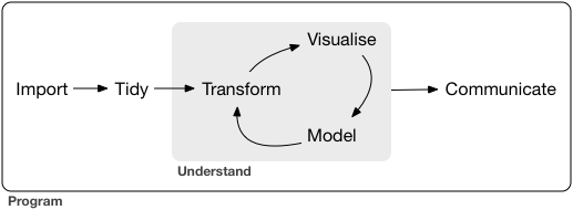
You can include your saved plot, or any image by using knitr::include_graphics in you R-chunk. E.g. if you include this line of code:
{r out.width = "75%", fig.cap = "From: Grolemund and Wickham"}
knitr::include_graphics("https://heima.hafro.is/~einarhj/crfmr_img/data_science.png")
you get this in your knitted document:
Spotting outlier (EH)
- Create a table with expected range of values
- Use that table to check you data entry to find records that are outside expected range:
library(tidyverse)
# Some imaginary trip data, here just one species caught per trip:
trip <-
  tibble(trip = 1:10,
         sid = c(rep("cod", 5), rep("haddock", 5)),
         kg = c(100, 90, 140, 300, 1000, 1, 9, 14, 30, 100))
# another table with upper bound on expected kg
expected_range <-
  tibble(sid = c("cod", "haddock"),
         upper = c(500, 50))
trip |>
  left_join(expected_range) |>
  mutate(outlier = ifelse(kg > upper, "check", "ok"))
# A tibble: 10 × 5
trip sid kg upper outlier
<int> <chr> <dbl> <dbl> <chr>
1 1 cod 100 500 ok
2 2 cod 90 500 ok
3 3 cod 140 500 ok
4 4 cod 300 500 ok
5 5 cod 1000 500 check
6 6 haddock 1 50 ok
7 7 haddock 9 50 ok
8 8 haddock 14 50 ok
9 9 haddock 30 50 ok
10 10 haddock 100 50 check ggplot-plotly (EH)
Supposedly any ggplot can be passed to plotly to generate an interactive graph. Following is a short example:
library(tidyverse)
library(plotly)

# A ggplot object.
p <-
  "ftp://ftp.hafro.is/pub/data/csv/minke.csv" |>
  read_csv() |>
  ggplot(aes(x = age, y = length)) +
  geom_point()
# turn a ggplot object into plotly
ggplotly(p)
On functions and arguments (EH)
Almost all the stuff you do in R is via some function call. All functions of course have a specific name and most functions have one or more arguements. A typical structure of a function looks something like this:
function_name(argument1 = value1, argument2 = value2, ...)Lets look at the function mean
help(mean)| mean | R Documentation |
Arithmetic Mean
Description
Generic function for the (trimmed) arithmetic mean.
Usage
mean(x, ...)

## Default S3 method:
mean(x, trim = 0, na.rm = FALSE, ...)
Arguments
x |
An R object. Currently there are methods for
numeric/logical vectors and date,
date-time and time interval objects. Complex vectors
are allowed for |
trim |
the fraction (0 to 0.5) of observations to be
trimmed from each end of |
na.rm |
a logical evaluating to |
... |
further arguments passed to or from other methods. |
Value
If trim is zero (the default), the arithmetic mean of the
values in x is computed, as a numeric or complex vector of
length one. If x is not logical (coerced to numeric), numeric
(including integer) or complex, NA_real_ is returned, with a warning.
If trim is non-zero, a symmetrically trimmed mean is computed
with a fraction of trim observations deleted from each end
before the mean is computed.
References
Becker, R. A., Chambers, J. M. and Wilks, A. R. (1988) The New S Language. Wadsworth & Brooks/Cole.
See Also
weighted.mean, mean.POSIXct,
colMeans for row and column means.
Examples
x <- c(0:10, 50)
xm <- mean(x)
c(xm, mean(x, trim = 0.10))
In the documentation we see that there are arguments like:
- x
- trim: Take note that the arguement is set to 0 by default
- na.rm: Take note that the arguement is set to FALSE by default
So when we use this function we need to specify some values for at least some of these arguments, e.g.:
mean(x = v_lengths)           # explicitly type the argument name (here x)
mean(v_lengths)               # do not type the arguement name, just use the argument order
mean(v_weights, na.rm = TRUE) # overwrite the default value set for the arguement na.rm
mean(v_weights, 0.4, TRUE)
When running the last command the value 0.4 is assigned to the arguement trim. If were to do this in the following order we get an error:
mean(v_weights, TRUE, 0.4)because the second arguement (trim) has to be numeric not a boolean and vica versa for the third arguement (na.rm). This would though not give an error because we explicitly name the argument:
mean(v_weights, na.rm = TRUE, trim = 0.4)On base R vs tidyverse (EH)
So far we have been dealing with data-frames (e.g. the minke data):
library(tidyverse)
w <- read_csv("ftp://ftp.hafro.is/pub/data/csv/minke.csv")
We can check the class of the object w via:
class(w) # key thing for now is that we see this is a "data.frame"[1] "spec_tbl_df" "tbl_df" "tbl" "data.frame" We access the values of each of the variables by using the ‘$’-sign:
w$length [1] 780 793 858 567 774 526 809 820 697 777 739 542 508 754 797 802 840 761
[19] 819 836 764 774 778 716 727 813 684 737 792 853 852 685 745 712 502 793
[37] 835 634 771 772 750 718 603 775 861 692 845 693 520 809 762 760 810 840
[55] 730 778 729 782 840 770 776 777 802 727 564 737 860 752 764 708 599 730
[73] 682 725 474 871 825 740 853 762 788 705 775 482 797 740 870 766 720 566
[91] 704 760 790 820 790 775 606 794 819 761 461 803 804 606 768 763 797 700
[109] 750 661 706 782 763 805 770 750 802 699 748 783 759 706 647 739 834 603
[127] 745 764 779 835 840 820 781 858 835 772 780 751 692 857 732 833 740 750
[145] 700 795 730 836 789 740 796 850 662 755 715 784 780 871 687 716 760 819
[163] 800 779 741 785 810 845 622 775 809 755 833 792 758 790 806 840 704 773
[181] 717 735 814 682 840 838 731 803 701 802w$weight [1] NA NA NA NA NA NA NA NA NA NA NA NA NA NA NA
[16] NA NA NA NA NA NA 4620 NA NA NA NA NA NA NA NA
[31] NA NA NA NA NA NA NA NA NA NA NA NA NA NA NA
[46] NA NA NA NA NA NA NA NA NA NA NA NA NA NA NA
[61] NA NA NA NA NA NA NA NA NA NA NA NA NA NA NA
[76] NA NA 3691 NA 3528 NA 2870 5328 NA 4848 NA NA 4260 3462 1663
[91] NA NA NA 5620 NA NA NA NA NA NA NA NA NA NA NA
[106] NA NA NA NA NA NA NA NA NA NA NA NA NA NA NA
[121] NA NA NA NA NA NA NA NA NA NA NA NA NA NA NA
[136] NA NA NA NA NA 3216 NA 3682 4350 NA NA NA NA NA NA
[151] NA NA NA 3182 NA NA NA NA NA NA NA NA NA NA NA
[166] NA NA NA NA NA NA NA NA NA NA NA NA NA NA NA
[181] 4062 3361 4520 4165 5301 5685 4358 NA NA NAWe can even access individual or sets of values using the ‘[ ]’
w$length[1] # length value of the first observations[1] 780w$weight[2] # weight value of the second observation[1] NAw$maturity[1:10] # maturity stage of the first 10 observations [1] "pregnant" "pregnant" "pregnant" "immature" "immature" "immature"
[7] "pregnant" "pregnant" "pubertal" "mature" In the Transformation-tutorial we calculated new variables within the data-frame, e.g. when calculating derived weight from length:
w |>
  mutate(computed_weight = 0.00001 * length^3)
We could have achieved the same thing by doing:
w$computed_weight <- 0.00001 * w$length^3We could even have “extracted” the lengths in the data-frame into a separate object (a numerical vector) and then done this:
v_lengths <- w$length
class(v_lengths)
[1] "numeric"v_weights <- w$weight
v_weights_computed <- 0.00001 * v_lengths^3What we have now though is a separate object for the derived weights and the only linkage between length and weights is the order within each vector, e.g. the fifth observations for length and then the derived weight can be obtained by:
v_lengths[5]
v_weights[5]
We can easily apply summary functions on these vectors, e.g.:
mean(v_lengths)
sd(v_lengths)
mean(v_weights, na.rm = TRUE)   # overwrite the default argument (see below)
sd(v_weight, na.rm = TRUE)      # overwrite the default argument (see below)
The above is an example of operation within the base-R environment
Why are you telling me this?:
- As you progress in R and start to look at other peoples code you are bound to stumble on base-R code like this.
- Although you can do a lot within the tidyverse-framework you will at some time need to know and use base-R.
- Think of base-R as your friend, not a foe.
Flying fish catch (EH)
library(tidyverse)
fao <- read_csv("https://heima.hafro.is/~einarhj/data/fao-capture-statistics_area31.csv")
fao |>
  filter(str_starts(species, "Fly")) |>
  ggplot(aes(year, catch, fill = country)) +
  geom_col() +
scale_fill_brewer(palette = "Set1") 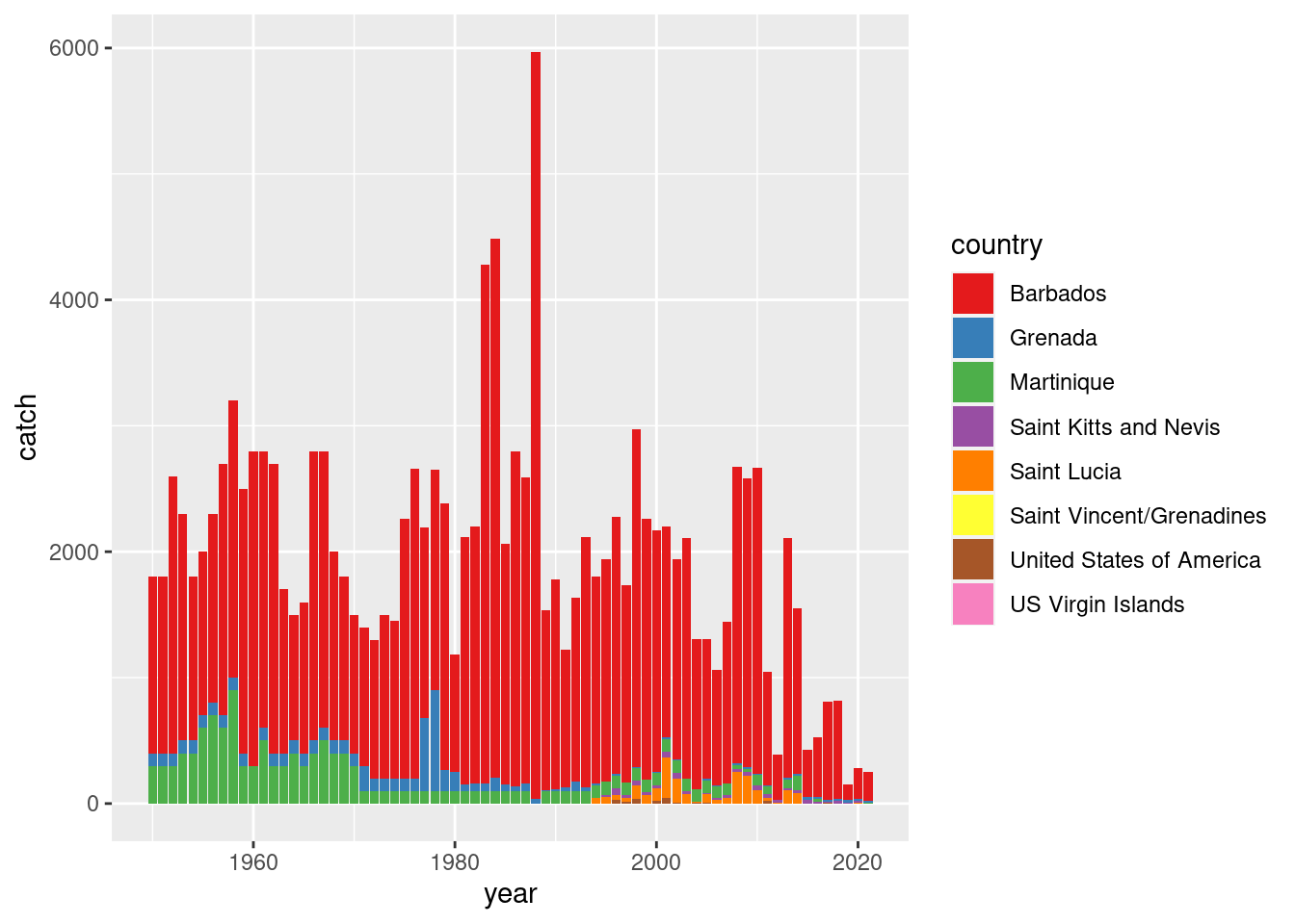
fao |>
  filter(str_starts(species, "Fly")) |>
  group_by(year) |>
  summarise(catch = sum(catch, na.rm = TRUE)) |>
  ggplot(aes(year, catch)) +
  geom_point() +
  geom_smooth() +
scale_x_continuous(breaks = seq(1950, 2020, by = 5)) 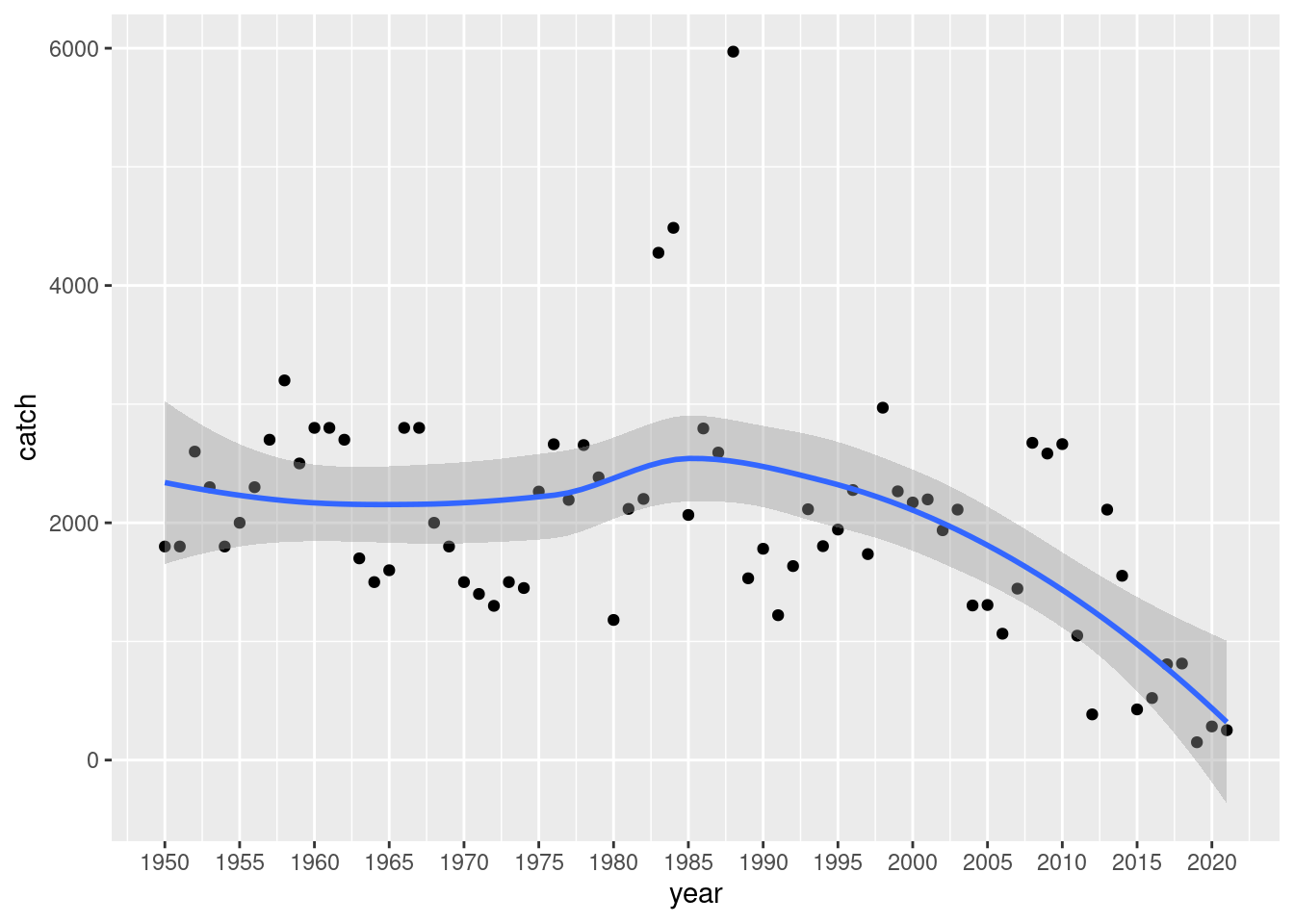
Dates (EH)
Your friend for working with dates and time are functions in the {lubridate}-package (automatically loaded when runinng library(tidyverse)). To get started, you can get some information by typing:
vignette(topic = "lubridate")And of course check chapter 18 Dates and times in the r4d-book.
A quick demo script:
- If you have dates in character form use one of
ymd-,dmy- ormdy-functions to get it into class “Date”. - Have the date in the right format one can then extract the year, month and day by functions of the same name
tibble(date_as_text = "13-jan-22") |>
  mutate(date = dmy(date_as_text),
         year = year(date),
         month = month(date),
         day = day(date))
# A tibble: 1 × 5
date_as_text date year month day
<chr> <date> <dbl> <dbl> <int>
1 13-jan-22 2022-01-13 2022 1 13CMSY download (EH)
download.file("https://oceanrep.geomar.de/id/eprint/52147/4/UserGuideCodeDataMarch2021.zip",
              mode = "wb",
              destfile = "CMSY.zip")
unzip(zipfile = "CMSY.zip")
In order to get the plots when doing just an ad-hoc File -> Complile report you may consider turning “close.plots <- F” to “close.plots <- T” in the general settings in CMSY R-script:
#-----------------------------------------
# General settings for the analysis ----
#-----------------------------------------
CV.C         <- 0.15  #><>MSY: Add Catch CV
CV.cpue      <- 0.2 #><>MSY: Add minimum realistic cpue CV
sigmaR       <- 0.1 # overall process error for CMSY; SD=0.1 is the default
cor.log.rk   <- -0.76 # empirical value of log r-k correlation in 250 stocks analyzed with BSM (without r-k correlation), used only in graph
rk.cor.beta  <- c(2.52,3.37) # beta.prior for rk cor+1
nbk          <- 3 # Number of B/k priors to be used by BSM, with options 1 (first year), 2 (first & intermediate), 3 (first, intermediate & final bk priors)
bt4pr        <- F # if TRUE, available abundance data are used for B/k prior settings
auto.start   <- F # if TRUE, start year will be set to first year with intermediate catch to avoid ambiguity between low and high bimass if catches are very low
ct_MSY.lim   <- 1.21  # ct/MSY.pr ratio above which B/k prior is assumed constant
q.biomass.pr <- c(0.9,1.1) # if btype=="biomass" this is the prior range for q
n            <- 5000 # number of points in multivariate cloud in graph panel (b)
ni           <- 3 # iterations for r-k-startbiomass combinations, to test different variability patterns; no improvement seen above 3
nab          <- 3 # recommended=5; minimum number of years with abundance data to run BSM
bw           <- 3 # default bandwidth to be used by ksmooth() for catch data
mgraphs      <- T # set to TRUE to produce additional graphs for management
e.creep.line <- T # set to TRUE to display uncorrected CPUE in biomass graph
kobe.plot    <- T # set to TRUE to produce additional kobe status plot; management graph needs to be TRUE for Kobe to work
BSMfits.plot <- T # set to TRUE to plot fit diagnostics for BSM
pp.plot      <- T # set to TRUE to plot Posterior and Prior distributions for CMSY and BSM
rk.diags     <- T #><>MSY set to TRUE to plot diagnostic plot for r-k space
retros       <- F # set to TRUE to enable retrospective analysis (1-3 years less in the time series)
save.plots   <- T # set to TRUE to save graphs to JPEG files
close.plots  <- F # set to TRUE to close on-screen plots after they are saved, to avoid "too many open devices" error in batch-processing
write.output <- T # set to TRUE if table with results in output file is wanted; expects years 2004-2014 to be available
write.pdf    <- F # set to TRUE if PDF output of results is wanted. See more instructions at end of code.
select.yr    <- NA # option to display F, B, F/Fmsy and B/Bmsy for a certain year; default NA
write.rdata  <- F #><>HW write R data file
Installing from github (EH)
# install.packages("devtools") # you may need this
devtools::install_github("debinqiu/snpar")