Summarizing and plotting length data

This document has some pointers on how to plot length data using a hypothetical data set. The data set represents a snapshot of length measurements in time for 2 months, for 1 species at 1 landing site for 1 year.

length_data <- read_csv("https://heima.hafro.is/~einarhj/crfmr/aux/length_exampledata.csv")

head(length_data)

# A tibble: 6 × 6
   year month   day landingsite speciesID length
  <dbl> <dbl> <dbl> <chr>           <dbl>  <dbl>
1  2014     4    26 A                   1     17
2  2014     4    26 A                   1     17
3  2014     4    26 A                   1     17
4  2014     4    26 A                   1     17
5  2014     4    26 A                   1     17
6  2014     4    26 A                   1     17

If one wishes to assign a bin to the data, the `cut` function can be used where the minimum and maximum observed lengths can be specified with a desired bin.

length_bin <- length_data %>% 
  mutate(bin = cut(length, seq(min(length), max(length) + 5, 5), right = FALSE))

Normally, one check do a count of the measurements to gather the numbers observed by each length measurement to get a frequency by length measurement.

length_count <- length_data %>% 
  group_by(year, month, landingsite, speciesID) %>% 
  count(length) %>% 
  as_tibble()

head(length_count)

# A tibble: 6 × 6
   year month landingsite speciesID length     n
  <dbl> <dbl> <chr>           <dbl>  <dbl> <int>
1  2014     3 A                   1     10    22
2  2014     3 A                   1     11    10
3  2014     3 A                   1     13    24
4  2014     3 A                   1     14    19
5  2014     3 A                   1     15    27
6  2014     3 A                   1     16    51

Proportions, assigned to `p` below can be calculated by year using simple math.

length_prop <-
  length_count %>%
  group_by(year) %>%
  mutate(p = n / sum(n) * 100) %>% 
  as_tibble()

head(length_prop)

# A tibble: 6 × 7
   year month landingsite speciesID length     n     p
  <dbl> <dbl> <chr>           <dbl>  <dbl> <int> <dbl>
1  2014     3 A                   1     10    22 0.974
2  2014     3 A                   1     11    10 0.443
3  2014     3 A                   1     13    24 1.06 
4  2014     3 A                   1     14    19 0.841
5  2014     3 A                   1     15    27 1.20 
6  2014     3 A                   1     16    51 2.26

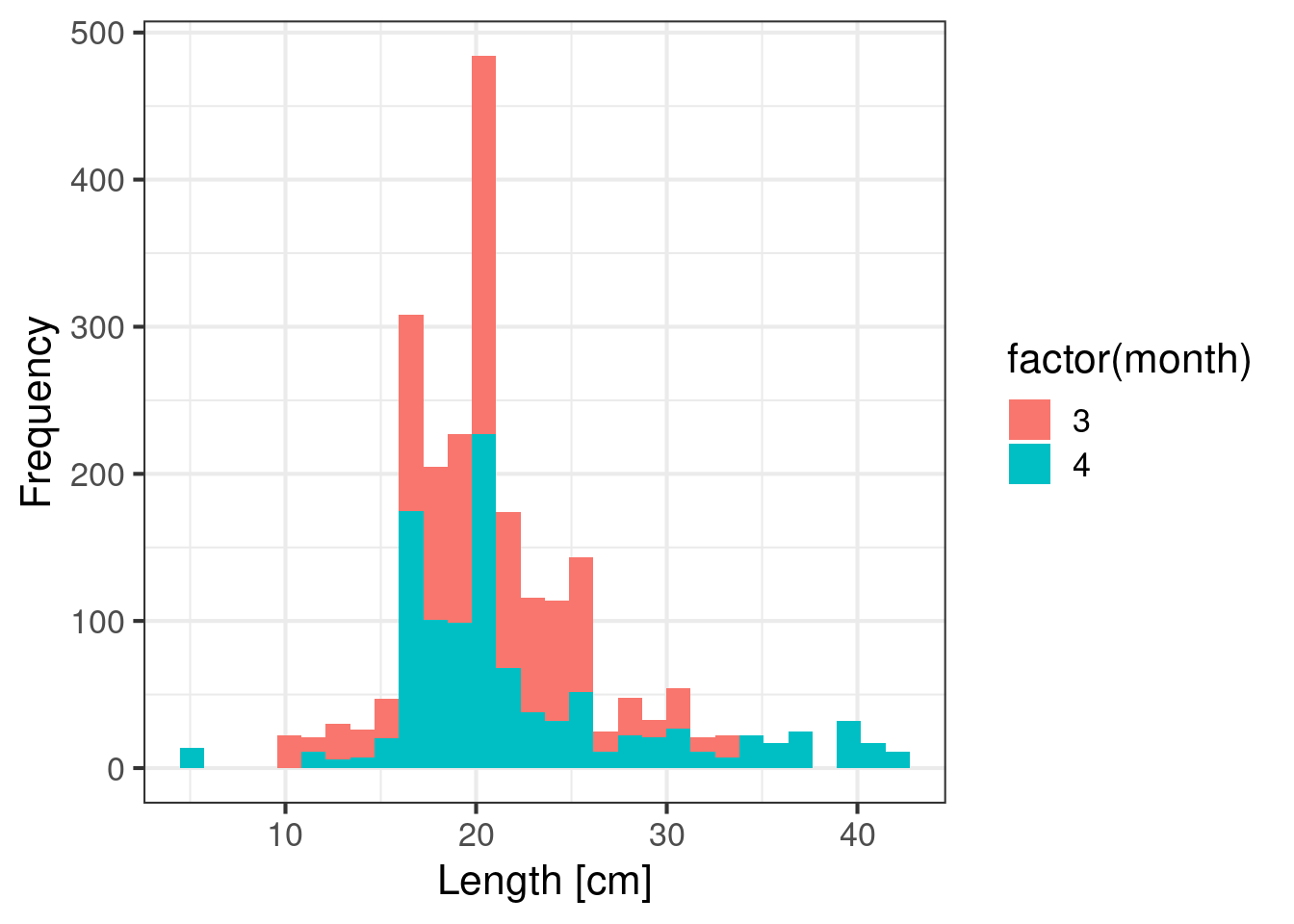
To visualize the distribution in length measurements, one can use the original data setup and compare by months, years, landing sites. The `scale_x_continuous` can be used adjust the x axis marks.

length_data %>%
  ggplot(aes(length, fill = factor(month))) +
  theme_bw(base_size = 16) +
  geom_histogram() +
  scale_x_continuous(breaks = seq(0, 50, by = 10)) +
  labs(x = "Length [cm]", y = "Frequency",
       colour = "Year")

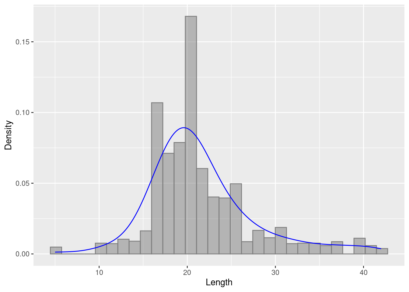
A density approach can also be used to visualize the data.

ggplot(length_data, 
       aes(length)) + 
  geom_histogram(aes(y=after_stat(density),), position="identity", alpha=0.5, col='grey50', fill='grey50')+
  geom_density(aes(length),adjust=2.5,color='blue') +
  ylab("Density") + xlab("Length")

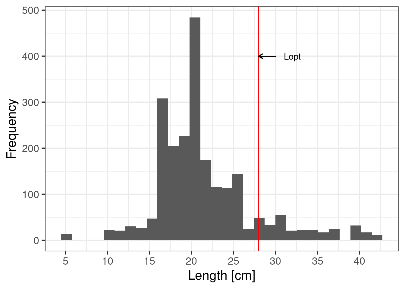
Below is an example code, showing how to overlay reference points on the plot and include text to make the distribution for descriptive using `geom_vline`,`geom_segment`and `annotate`.

Lopt <- 28
 
length_data %>%
  ggplot(aes(length)) +
  theme_bw(base_size = 16) +
  geom_histogram() +
  scale_x_continuous(breaks = seq(0, 50, by = 5)) +
  labs(x = "Length [cm]", y = "Frequency",
       colour = "Year") +
  geom_vline(aes(xintercept = Lopt), color = "red",
             linetype = "solid", size = 0.5) +
  geom_segment(aes(x = 30, y = 400, xend = 28, yend = 400),
               arrow = arrow(length = unit(0.2, "cm"))) +
  annotate("text", x = 32, y = 400, label = "Lopt")

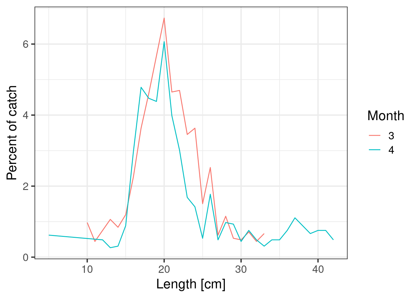
One also normally uses `geom_line` to visualize length frequency. This is rather noisy because the data set is small.

length_prop %>% 
  ggplot(aes(length, p, color = factor(month))) +
  theme_bw(base_size = 16) +
  geom_line() +
  scale_x_continuous(breaks = seq(0, 50, by = 10)) +
  labs(x = "Length [cm]", y = "Percent of catch",
       colour = "Month")

Find ways to make this prettier and more informative.