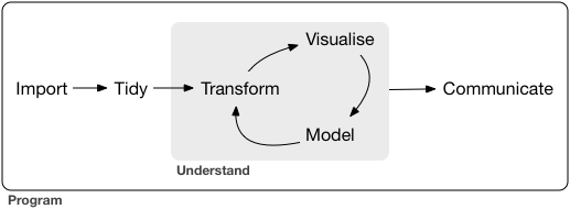
Transformation
Preamble
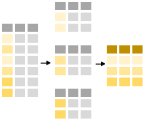
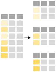
Commonly, when collating summaries by group, one wants to:
- Split up a big data structure into homogeneous pieces,
- Apply a function to each piece
- Combine all the results back together.
For example, one might want to:
- Calculate summary statistics for each category (read: group)
- Perform group-wise transformations (read: apply) like summary or re-scaling/standardization
- Fit the same model to different subset of the data
The tidyverse package, through the dplyr, comes to the rescue.
- Similar to ggplot2 they feature a Domain Specific Language (DSL) specially designed for data summaries.
- Developed by Hadley Wickam, the creator ggplot2 and other useful tools.
Essentially dplyr offer a collection of simple but powerful commands (think of them as verbs) that facilitate this process:
- filter: keep observations (rows) matching criteria
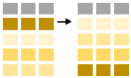
- select: pick variables (columns) by name
- arrange: order the observations (rows) according to a variable (column)
- mutate: add new or modify existing variables (column)
- summarise: reduce variables to some summary values
- group_by: gives the group to apply the analysis functions to
The structure of these commands is always the same:
- First argument to the function is a data frame
- Subsequent arguments say what to do with data frame, typically what variables to operate on.
- Always return a data frame
- this is the key difference of the tidyverse vs. base R approach
- It recognizes the variables (columns) of the data.frame as variables, that is one only need to write
variable_nameinstead ofdat$variable_name
Each of the main dplyr-functions normally does one thing only (but does it “well”) so one normally uses a combination of the above functions. Below we will jump right into using the pipe (|> or %>%).
Reading material
The pipe
We need to load the library {tidyverse} into our current session and we will use the minke-data for demonstation:
library(tidyverse)
w <-
  "ftp://ftp.hafro.is/pub/data/csv/minke.csv" |>
  read_csv()
The code structure above is a little bit different than used up to now:
w <- read_csv("ftp://ftp.hafro.is/pub/data/csv/minke.csv")and is just to gently introduce you to the |>-concept (often read as: “pipe”-concept) that needs a bit of extra explaining:
- Noticed that the first argument (“file”) in
read_csvin the first code-chunk is missing. Writing justread_csv()on its own would give you an error: ‘argument “file” is missing, with no default’. - The
|>operator takes the stuff on the left (here actually in the line above) and places it as the first argument to function on the right hand side.
Recomended that you “read” the |> as “then”. Hence the above can be read as:
- create a text string “ftp://ftp.hafro.is/pub/data/csv/minke.csv”.
- then (
|>) pass it as the first argument into the next function (read_csv).
- Some notes on function and arguments can be found here.
- store the data in object “w” (here declared in the first line).
Some even go the whole way in code-writing from “left-to-right”, like:
"ftp://ftp.hafro.is/pub/data/csv/minke.csv" |>
  read_csv() ->
  w
Note that Rstudio has a built in shortcut for the |> operator: [ctrl] + [shift] + M.
Operation on observations (rows)
filter: Extract observations
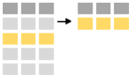
One can extract observations that meet logical criteria by using the filter command. The first argument is the name of the data frame with subsequent argument(s) being logical expressions. E.g. one subsets the minke data containing only year 2004 (the years in the dataset are from 2003 to 2007) by:
w |> filter(year == 2004)# A tibble: 25 × 13
id date lon lat area length weight age sex
<dbl> <dttm> <dbl> <dbl> <chr> <dbl> <dbl> <dbl> <chr>
1 1 2004-06-10 22:00:00 -21.4 65.7 North 780 NA 11.3 Female
2 690 2004-06-15 17:00:00 -21.4 65.7 North 793 NA NA Female
3 926 2004-06-22 01:00:00 -19.8 66.5 North 858 NA 15.5 Female
4 1430 2004-06-22 09:00:00 -19.8 66.5 North 840 NA 15.9 Female
5 1432 2004-06-26 05:00:00 -19.6 65.9 North 761 NA 14 Female
6 1434 2004-07-04 16:00:00 -21.0 65.5 North 819 NA 16.6 Female
7 1435 2004-06-04 19:00:00 -22.5 64.6 South 836 NA 46.8 Male
8 1437 2004-06-15 13:00:00 -23.0 64.2 South 764 NA 9.9 Male
9 1439 2004-06-08 07:00:00 -22.8 64.6 South 774 4620 10.9 Female
10 1440 2004-06-16 11:00:00 -23.4 64.2 South 778 NA 25.3 Male
# ℹ 15 more rows
# ℹ 4 more variables: maturity <chr>, stomach.volume <dbl>,
# stomach.weight <dbl>, year <dbl>Same as:
w |> filter(year %in% 2004)Only data from 2004 and onwards:
w |> filter(year >= 2004)Filter observations by some interval:
w |> filter(year >= 2004, year < 2006)  # the "," here should be read as "and"
w |> filter(year >= 2004 & year < 2006) # same as above, here more explicit
w |> filter(between(year, 2004, 2005))  # same as above
All but the year 2004 would be:
w |> filter(year != 2004) # "!=" should be read as not equal tooBut this would give year 2005 to 2007:
w |> filter(year %in% 2005:2007)Which would be the same as:
filter(w, !year %in% 2003:2004) # again "!" stands for "not" in RFilter takes any logical statement:
x == a    # x is equal to a
x != a    # x is not equal to a
x %in% a  # x is "in" a
!x %in% a # x is "not in" a
x > a    # x is greater than a
x >= a   # x is greater or equal to a
x < a    # x is less than a
x <= a   # x is less or equal to a
a & b    # a and b
a | b    # a or b
is.na(x) # is a equal to NA (missing)
...      # ...
The arguments can operate on different variables. E.g. to extract mature males caught in 2007 one would write:
w |> filter(maturity == "mature", sex == "Male", year == 2007)
w |> filter(maturity == "mature" & sex == "Male" & year == 2007) # same thing, more explicit
NOTE: A “comma” is recognized as “AND”. If one were to specify “OR” use the “|”:
filter(w, maturity == "mature" | sex == "Male" | year == 2007)- Find all males caught in the northern area in 2006 and 2007
- Find all males that are either immature or pregnant
- Find all whales caught that did not have a maturity status determined
- Find all whales that were caught in year 2007 or were mature males
w |> filter(sex == "Male", area == "North", year %in% 2006:2007)
w |> filter(sex == "Male", maturity %in% c("immature", "pregnant"))
w |> filter(is.na(maturity))
w |> filter(year == 2007 | (maturity == "mature" & sex == "Male"))arrange: Order observations
To sort the data we employ the arrange-function. Sorting by length is as follows (in ascending order):
w |> arrange(length)# A tibble: 190 × 13
id date lon lat area length weight age sex
<dbl> <dttm> <dbl> <dbl> <chr> <dbl> <dbl> <dbl> <chr>
1 20927 2006-07-19 15:00:00 -19.2 66.3 North 461 NA 3.4 Female
2 20254 2005-08-10 16:00:00 -16.8 66.4 North 474 NA 3.4 Male
3 20421 2005-07-19 17:00:00 -15.9 64.1 South 482 NA 3.6 Male
4 1481 2004-07-03 09:00:00 -15.8 64 South 502 NA 6.7 Female
5 1344 2003-08-26 16:00:00 -19.3 66.2 North 508 NA NA Male
6 1504 2003-08-18 17:00:00 -23.9 65.0 South 520 NA 13.3 Male
7 1335 2003-09-16 16:00:00 -18.7 66.2 North 526 NA 9.6 Female
8 1343 2003-08-28 19:00:00 -15.8 66.4 North 542 NA NA Female
9 19211 2005-07-23 16:00:00 -14.2 65.8 North 564 NA 5.2 Female
10 20427 2005-08-03 15:00:00 -23.1 64.6 South 566 1663 6.1 Male
# ℹ 180 more rows
# ℹ 4 more variables: maturity <chr>, stomach.volume <dbl>,
# stomach.weight <dbl>, year <dbl>and in descending order:
w |> arrange(desc(length))You can also arrange by more that one column:
w |> arrange(sex, desc(length))Above first orders the data by sex (alphabetical, first Female then Male) and then by increasing length.
distinct
distinct can be used extract unique observations in a data frame. The command below would operate on all the variables in the dataframe (so if there were duplicate observations you would only get unique records):
w |> distinct()The minke data actally has distinct records so the above example is a bit meaningless. One however normally operates on selected variables like:
w |> distinct(sex)# A tibble: 2 × 1
sex
<chr>
1 Female
2 Male w |> distinct(sex, maturity) # so no record of a pregnant male!# A tibble: 8 × 2
sex maturity
<chr> <chr>
1 Female pregnant
2 Male immature
3 Female immature
4 Male pubertal
5 Male mature
6 Female anoestrous
7 Female <NA>
8 Male <NA> If we wanted to get the distinct records in a particular order we could do:
w |>
  distinct(sex, maturity) |>
  arrange(sex, maturity)
# A tibble: 8 × 2
sex maturity
<chr> <chr>
1 Female anoestrous
2 Female immature
3 Female pregnant
4 Female <NA>
5 Male immature
6 Male mature
7 Male pubertal
8 Male <NA> This is an example of combining the dplyr-functions in a single pipe-flow, something we will do a lot of in this course.
Operations on variables (columns)
select: Extract variables
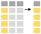
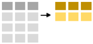
The select functions allows you to extract certain variables of interest.
Select columns by name:
w |> select(id, sex, maturity)# A tibble: 190 × 3
id sex maturity
<dbl> <chr> <chr>
1 1 Female pregnant
2 690 Female pregnant
3 926 Female pregnant
4 1333 Male immature
5 1334 Female immature
6 1335 Female immature
7 1336 Female pregnant
8 1338 Female pregnant
9 1339 Male pubertal
10 1341 Male mature
# ℹ 180 more rowsSelect all columns between length and age:
w |> select(length:age)You can also omit certain columns using negative indexing: for example you can select all columns except those between sex and stomach.weight
w |> select(!sex:stomach.weight)# A tibble: 190 × 9
id date lon lat area length weight age year
<dbl> <dttm> <dbl> <dbl> <chr> <dbl> <dbl> <dbl> <dbl>
1 1 2004-06-10 22:00:00 -21.4 65.7 North 780 NA 11.3 2004
2 690 2004-06-15 17:00:00 -21.4 65.7 North 793 NA NA 2004
3 926 2004-06-22 01:00:00 -19.8 66.5 North 858 NA 15.5 2004
4 1333 2003-09-30 16:00:00 -21.6 65.7 North 567 NA 7.2 2003
5 1334 2003-09-25 15:00:00 -15.6 66.3 North 774 NA 12.3 2003
6 1335 2003-09-16 16:00:00 -18.7 66.2 North 526 NA 9.6 2003
7 1336 2003-09-12 17:00:00 -21.5 65.7 North 809 NA 17.3 2003
8 1338 2003-09-09 12:00:00 -22.8 66.1 North 820 NA 13.8 2003
9 1339 2003-08-31 13:00:00 -17.5 66.6 North 697 NA 12.2 2003
10 1341 2003-08-30 17:00:00 -14.7 66.2 North 777 NA 15.4 2003
# ℹ 180 more rowsA combination of non-adjacent variables to drop could be written as:
w |> select(-c(weight, maturity))You can select all categorical values by:
w |> select(where(is.character))# A tibble: 190 × 3
area sex maturity
<chr> <chr> <chr>
1 North Female pregnant
2 North Female pregnant
3 North Female pregnant
4 North Male immature
5 North Female immature
6 North Female immature
7 North Female pregnant
8 North Female pregnant
9 North Male pubertal
10 North Male mature
# ℹ 180 more rowsThe select function has some useful helper function:
starts_with('stomach')  # Finds all columns that start with "stomach"
ends_with('weight')     # Finds all columns that end with "weight"
contains('mach')        # Finds all columns that contain "mach"
And you can of course combine these at will:
w |> select(id, length, starts_with('stomach'))# A tibble: 190 × 4
id length stomach.volume stomach.weight
<dbl> <dbl> <dbl> <dbl>
1 1 780 58 31.9
2 690 793 90 36.3
3 926 858 24 9.42
4 1333 567 25 3.64
5 1334 774 85 5.51
6 1335 526 18 1.17
7 1336 809 200 99
8 1338 820 111 64.3
9 1339 697 8 0.801
10 1341 777 25 1.42
# ℹ 180 more rowsselect also allows you to rename columns as you select them:
w |> select(id, yr = year)# A tibble: 190 × 2
id yr
<dbl> <dbl>
1 1 2004
2 690 2004
3 926 2004
4 1333 2003
5 1334 2003
6 1335 2003
7 1336 2003
8 1338 2003
9 1339 2003
10 1341 2003
# ℹ 180 more rowsbut this only selects the requested columns, others are dropped.
rename: Rename columns
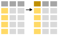
If you just want to rename a couple of columns in the data frame leaving the other columns intact you can use the function rename:
w |> rename(time = date, stomach_volume = stomach.volume)# A tibble: 190 × 13
id time lon lat area length weight age sex
<dbl> <dttm> <dbl> <dbl> <chr> <dbl> <dbl> <dbl> <chr>
1 1 2004-06-10 22:00:00 -21.4 65.7 North 780 NA 11.3 Female
2 690 2004-06-15 17:00:00 -21.4 65.7 North 793 NA NA Female
3 926 2004-06-22 01:00:00 -19.8 66.5 North 858 NA 15.5 Female
4 1333 2003-09-30 16:00:00 -21.6 65.7 North 567 NA 7.2 Male
5 1334 2003-09-25 15:00:00 -15.6 66.3 North 774 NA 12.3 Female
6 1335 2003-09-16 16:00:00 -18.7 66.2 North 526 NA 9.6 Female
7 1336 2003-09-12 17:00:00 -21.5 65.7 North 809 NA 17.3 Female
8 1338 2003-09-09 12:00:00 -22.8 66.1 North 820 NA 13.8 Female
9 1339 2003-08-31 13:00:00 -17.5 66.6 North 697 NA 12.2 Male
10 1341 2003-08-30 17:00:00 -14.7 66.2 North 777 NA 15.4 Male
# ℹ 180 more rows
# ℹ 4 more variables: maturity <chr>, stomach_volume <dbl>,
# stomach.weight <dbl>, year <dbl>- Select age, length and id from the minke dataset, and rename id to “whale_id”
- Select the id column and all columns that contain the text “weight”.
w |> select(age, length, whale_id = id)
w |> select(id, contains("weight"))mutate: Compute new variable
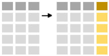
mutate allows you to add new columns to your data. Let’s calculate the approximate weight:
w |>
  select(id, length, weight) |>
  mutate(computed_weight = 0.00001 * length^3)
# A tibble: 190 × 4
id length weight computed_weight
<dbl> <dbl> <dbl> <dbl>
1 1 780 NA 4746.
2 690 793 NA 4987.
3 926 858 NA 6316.
4 1333 567 NA 1823.
5 1334 774 NA 4637.
6 1335 526 NA 1455.
7 1336 809 NA 5295.
8 1338 820 NA 5514.
9 1339 697 NA 3386.
10 1341 777 NA 4691.
# ℹ 180 more rowsYou can also do more than one “mutation”:
w |>
  select(id, length, weight) |>
  mutate(computed_weight = 0.00001 * length^3,
         weight2 = ifelse(is.na(weight), 0.00001 * length^3, weight))
# A tibble: 190 × 5
id length weight computed_weight weight2
<dbl> <dbl> <dbl> <dbl> <dbl>
1 1 780 NA 4746. 4746.
2 690 793 NA 4987. 4987.
3 926 858 NA 6316. 6316.
4 1333 567 NA 1823. 1823.
5 1334 774 NA 4637. 4637.
6 1335 526 NA 1455. 1455.
7 1336 809 NA 5295. 5295.
8 1338 820 NA 5514. 5514.
9 1339 697 NA 3386. 3386.
10 1341 777 NA 4691. 4691.
# ℹ 180 more rowsTo make our lives a bit easier mutate “remembers” earlier transformations within the sequence:
w |>
  select(id, length, weight) |>
  mutate(computed_weight = 0.00001 * length^3,
         approx_weight = ifelse(is.na(weight), computed_weight, weight))
One can also overwrite existing variables:
w |>
  select(id, length, weight) |>
  mutate(computed_weight = 0.00001 * length^3,
         weight = ifelse(is.na(weight), computed_weight, weight))
And even not create a temporary variable (here computed_weight):
w |>
  select(id, length, weight) |>
mutate(weight = ifelse(is.na(weight), 0.00001 * length^3, weight))Calculate the Fullton’s condition factor for whales where observations of weights exists. The formula is:
\(K=100(W/L^3)\)
Note: the weights need to be in grams, the length in cm
Hint: Use the function is.na (in the sense of !is.na) to filter out records with observed weight.
w |>
  filter(!is.na(weight)) |>
  select(id, length, weight) |>
  mutate(K = 100 * (1000 * weight / length^3))

# another way:
w |>
  select(id, length, weight) |>
  drop_na() |>
  mutate(K = 100 * (1000 * weight / length^3))
Summarise cases
summarise:
To summarise data one uses the summarise-function. Below we calculate the number of observations (using the cl("n")-function and the mean minke length.
w |>
  summarise(n.obs = n(),
            ml = mean(length, na.rm = TRUE))
# A tibble: 1 × 2
n.obs ml
<int> <dbl>
1 190 753.group_by:
The power of the command summarise is revealed when used in conjunction with group_by-function. The latter functions splits the data into groups based on one or multiple variables. E.g. one can split the minke table by maturity:
w |>
  group_by(maturity)
# A tibble: 190 × 13
# Groups: maturity [6]
id date lon lat area length weight age sex
<dbl> <dttm> <dbl> <dbl> <chr> <dbl> <dbl> <dbl> <chr>
1 1 2004-06-10 22:00:00 -21.4 65.7 North 780 NA 11.3 Female
2 690 2004-06-15 17:00:00 -21.4 65.7 North 793 NA NA Female
3 926 2004-06-22 01:00:00 -19.8 66.5 North 858 NA 15.5 Female
4 1333 2003-09-30 16:00:00 -21.6 65.7 North 567 NA 7.2 Male
5 1334 2003-09-25 15:00:00 -15.6 66.3 North 774 NA 12.3 Female
6 1335 2003-09-16 16:00:00 -18.7 66.2 North 526 NA 9.6 Female
7 1336 2003-09-12 17:00:00 -21.5 65.7 North 809 NA 17.3 Female
8 1338 2003-09-09 12:00:00 -22.8 66.1 North 820 NA 13.8 Female
9 1339 2003-08-31 13:00:00 -17.5 66.6 North 697 NA 12.2 Male
10 1341 2003-08-30 17:00:00 -14.7 66.2 North 777 NA 15.4 Male
# ℹ 180 more rows
# ℹ 4 more variables: maturity <chr>, stomach.volume <dbl>,
# stomach.weight <dbl>, year <dbl>The table appears “intact” because it still has 190 observations but it has 6 groups, representing the different values of the maturity scaling in the data (anoestrous, immature, mature, pregnant, pubertal and “NA”).
The summarise-command respects the grouping, as shown if one uses the same command as used above, but now on a dataframe that has been grouped:
w |>
  group_by(maturity) |>
  summarise(n.obs = n(),
            mean = mean(length))
# A tibble: 6 × 3
maturity n.obs mean
<chr> <int> <dbl>
1 anoestrous 6 784.
2 immature 25 619.
3 mature 74 758.
4 pregnant 66 800.
5 pubertal 6 692.
6 <NA> 13 752.- Calculate the number of observations and minimum, median, mean, standard deviation and standard error of whale lengths in each year
- The function names in R are:
- n
- min
- max
- median
- mean
- sd
The function for standard error is not availble in R. A remedy is that you use college statistical knowledge to derive them from the appropriate variables you derived above.
w |>
  group_by(year) |>
  summarise(n = n(),
            min = min(length),
            max = max(length),
            median = median(length),
            mean = mean(length),
            sd = sd(length),
            se = sd / sqrt(n))