Redfish

Some of the main characteristics are

1.

Simulation period is from 1970 to 1999. Two timesteps are used each year

2.

Natural mortality is set to 0.15 for the youngest decreasing gradually to 0.05 or 0.1 for age 5 and older.

3.

The ages used are 1 to 30 years. The oldest age is treated as a plus group.

4.

Recruitment was at age 1. Prior to 1989 length at recruitment was 7.1 cm but 8.1 cm afer that. This was supposed to reflect length of the 1985 and 1990 yearclasses in the groundfish survey.

3 alternatives were tested.

1.

M = 0.05

2.

Same as the first alternative but age readings were not used in the objective function

3.

M = 0.1

The solution found in alternative 2 was nearly identical to alternative 1. The optimizing algorithms had on the other hand much easier time finding the solution when the age readings were used. Here after only alternatives 1 and 3 will be discussed.

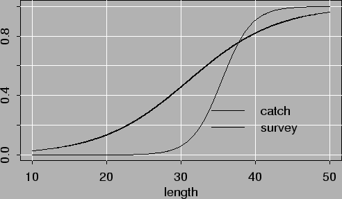
Figure 3.1 shows the estimated selection patterns of the commercial catch and the survey for alternative 1. Those estimated in alternative 3 were nearly identical.

  

Figure 3.1: Estimated selection pattern according to alternatives 1 and 3

Figure 3.2 shows estimated recruitment as age 1 according to model (M = 0.05). The main indicator for recruitment is the groundfish survey, which does not indicate that anything is on the way after the 1990 yearclass. Here the 1990 yearclass seems somewhat smaller than the 1985 yearclass. Much less data are available to estimate the recruitment prior to 1985.

If M = 0.1 is assumed half of the 1990 yearclass is moved to 1991 (figure 3.3) to compensate for faster growth (figure 3.4). If the model was allowed to estimate length at recruitment is used 6 cm for the 1990 yearclass which is shorter than survey data indicates. When M = 0.05 similiar things happen but the 1991 yearclass then becomes much less. The solution to this problem is probably to use more flexible growth model than the von Bertalanfy's equation. In the model this can for example be implemented by splitting the stock in mature and immature parts, with seperate growth parameters.

  

Figure 3.2: Estimated recruitment accoring to the model (M = 0.05)

  

Figure 3.3: Estimated recruitment accoring to the model (M = 0.1)

  

Figure 3.4: Estimated growth of redfish using

  

Figure 3.5: Estimated yield per recruit g/age 1 recruit according to model

Figure 3.4 shows the mean length of redfish including and without commercial catch The figure shows that the catch has much effect on mean length at age of older fish. The dotted lines in the figure are one standard deviation from the mean. Comparing figure 3.4 with the selection pattern indicates that each yearclass takes many years to recruit to the catchable stock.

Figure 3.4 also shows the estimated growth when M=0.1 is assumed. The growth is then more in the beginning but $L_{\inf}$ is less (54 vs. 62 cm).

Table 3.1 shows the distribution of the objective function on different components. Using M=0.1 gave a better fit to the data than using M=0.05 Plotting yield per recruit gave F_0.1 0.086 for alternative 1 and 0.156 for alternative3. F_max were on the other hand 0.16 and 0.37 (Figure 3.5).

 

Table 3.1: Distribution of the objective function

name	alt1	%alt1	alt3	%alt3
Length distribution in catch 72-84	32388.00	10.10	33150.00	10.49
Length distribution in catch 85-98	110030.00	34.31	105740.00	33.47
Understocking	0.00	0.00	0.00	0.00
Age length keys	31980.00	9.97	25900.00	8.20
Bounds	0.00	0.00	0.00	0.00
Mean length at age	73200.00	22.83	79950.00	25.30
Survey indices 11-24 cm	15180.00	4.73	15360.00	4.86
Survey indices 55-42 cm	47940.00	14.95	45080.00	14.27
Suvvey indices 5-10 cm	9799.00	3.06	10590.00	3.35
survey.ldr	128.50	0.04	143.80	0.05
total	320645.50	100.00	315913.80	100.00

 

Figures 3.6 to 3.7 show the development of the stock and catches when F_0.1 is used after 1998.

  

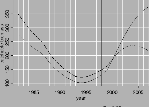
Figure 3.6: Development of catchable biomass of redfish using F_0.1after 1998. Solid line is for M = 0.05 and dotted line for M = 0.1

  

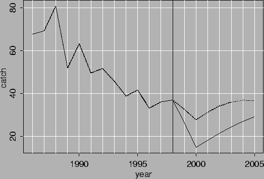
Figure 3.7: Development of catches of redfish using F_0.1 after 1998. Solid line is for M = 0.05 and dotted line for M = 0.1

As may be seen the catches will be steady in the nearest future if M=0.1 is a correct assumption. If M=0.05 is correct the catches should be decreased if F=F_0.1 is the catch rule. Figures 3.8 and 3.9 show development of the catches in near future for 4 different values of F. The lowest F is close to F_max (figure 3.5). In all cases the catchable biomass increases in the beginning but starts to decrease late in the period. If the groundfish survey is to be accepted as a measure of recruitment no new yearclass will show up in the catch until 2010 so the 1985 and 1990 yearclasses need to be preserved at least until then.

  

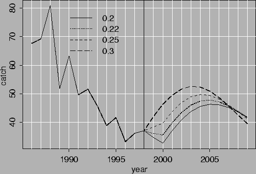
Figure 3.8: Development of catches of redfish with M = 0.05 using 4 different values of F As usually F means here the F of the largest fish with selection close to 1.

  

Figure 3.9: Development of catchable biomass of redfish with M = 0.05 using 4 different values of F