Plaice

Some of the main characteristics are

• The simulation period is from 1982 to 1999. Four timesteps are used each year
• Natural mortality is set to 0.15
• The age used is 2 to 15 years. The oldest age is not a plus group.

Prior to 1995 relatively few plaices were sampled from commercial catch but since then sampling has been more extensive. One problem with the samples is that much more otholiths have been sampled from Faxabay than its share in catches justifies. Therefore samples from Faxabay got less weight (1/3) than samples in other areas.

Plaice is caught at more than 200 stations in the Icelandic groundfish survey. The survey indices look fairly consistent with steep collapse from 1985 to 1994 (the survey started 1985) but have been relatively steady since 1994, even showing a slight upward trend in the last year. Still the index of catchable biomass today is only around 10% of what it was in 1985.

Otholith samples from the survey are available from 3 years 1987, 1990 and 1991. They are used in the objective function.

Five alternatives were tested.

1.

Not using survey indices.

2.

Using length disaggregated survey indices. Nonlinear relatioship between survey indices and stock size was allowed

3.

Using length disaggregated survey indices. Linear relatioship between survey indices and stock size assumed

4.

Using length disaggregated survey indices. Linear relatioship between survey indices and stock size assumed. More weight given to survey indices than in alternative 3

5.

Using length disaggregated survey indices. Linear relatioship between survey indices and stock size assumed. Survey indices from 1985 and 1986 are not used

In all cases length distributions and age length keys from the survey are included.

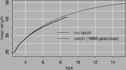
Figures 2.1 and 2.2 show the estimated growth and selection pattern for alternative 2. Figure 2.1 demonstrates the effect of the catch on mean length at age. The effect will be more today when fishing mortality is higher. Figure 2.3 shows yield per recruit based on the estimated growth and selection curves. The values of F_max and F_0.1 are 0.25 and 0.45 respectively.

  

Figure 2.1: Growth of plaice according to the model, with no catch and with mortality according to alternative 2

  

Figure 2.2: Estimated selection pattern of survey and commercial fleet from alternative 2

  

Figure 2.3: Yield as function of fishing mortality using parameters estimated in alternative 2

2.4 show the recruitment at age 3 for alternatives 2 and 3. As may be seen recuitment in recent years is much better according to alternative 2. Alternatives 1, 4 and 5 give similar picture to alternative 2.

  

Figure 2.4: Recruitment at age 3 for alternatives 2 and 3

Figures 2.5, 2.7 and 2.6 show the development of the fishing mortality, catches and catchable biomass using F=0.25 after 1998. Recruitment of yearclasses 1996 to 1998 was set to 13 million for all alternatives. This is higher than the estimate of the 1996 yearclass in alternative 1,3,4 and 5 but lower than in alternative 2. (figure 2.4)

Loooking at the results alternatives 1,3,4 and 5 all show similar trend while alternative 2 which allows nonlinear relationship between survey indices and stock size, gives more optimistic picture in recent years.

  

Figure 2.5: Fishing mortality of age 7 plaice. F = 0.25 after 1998

  

Figure 2.6: Biomass of age 5+ plaice. F = 0.25 after 1998

  

Figure 2.7: Development of catches. F = 0.25 after 1998

Figures 2.9 and 2.8 show the development of the catches and catchable biomass using alternative 3 and the same recruitment as before.

  

Figure 2.8: Biomass of age 5+ plaice alternative 3. F = 0.25,0.3,0.35,0.4

  

Figure 2.9: Development of catches for different values of F (alternative 3) F = 0.25,0.3,0.35,0.4

The final and most important question is then what to belive, alternative 2 or some of the other alternatives. Table 2 shows the objective function for alternatives 1, 2 and 3 and table 2.2 shows some information regarding survey indices for alternatives 2 and 3. SSE in the fit of survey indices vs. stock size is usually considerably lower in alternative 2 (as expected) but the power in the nonlinear relationship is extremely high. Table 2 shows that much weight is placed on samples from commercial catches. (Age length keys and length distributions).

 

Table 2.1: Distribution of the objective function for alternatives 1, 2 and 3.

Component	alt1	alt2	alt3	%alt1	%alt2	%alt3
Understocking	0.00	0.00	0.00	0.00	0.00	0.00
Alkeys catch	39198.00	39546.00	39420.00	26.08	23.59	23.06
Alkeys Survey	5531.00	5107.00	5428.00	3.68	3.05	3.17
Bounds	0.00	0.00	43.06	0.00	0.00	0.03
Length distr catch	75448.00	77108.00	76264.00	50.19	45.99	44.60
Length distr autumn survey	5626.50	5820.00	5887.50	3.74	3.47	3.44
Length distr survey	15270.00	17085.00	16020.00	10.16	10.19	9.37
Mean length in catch8	2397.15	2072.85	2222.05	1.59	1.24	1.30
Mean length in survey	6848.00	6996.00	7112.00	4.56	4.17	4.16
Survey indices 20-35cm		11450.00	13610.00		6.83	7.96
Survey indices 40-50cm		2482.00	4973.00		1.48	2.91

 

 

Table 2.2: SSE and power b in the equation I = aN^b for alternatives 2 and 3. b is always 1 in alternative 3

lengthgroup	17-22	23-28	28-32	33-37	38-42	43-47	48-52
SSE alternative 3	5.43	4.31	1.61	2.23	1.71	1.76	1.62
SSE alternative 2	4.63	4.14	1.32	1.38	0.66	1.03	1.16
power alternative 2	2.11	1.55	2.70	2.80	2.20	1.70	1.50