Case example 1
Mendo et al 2019
case_example01.RmdPremble
The code presented here is a modification of the code in supplement to “Identifying fishing grounds from vessel tracks: model-based inference for small scale fisheries” by Tania Mendo, Sophie Smout, Theoni Photopoulou and Mark James (2019) Royal Society Open Science. The supplementary document provides a code for “five different methods for identifying hauling versus non-hauling activities in small scale fishing vessels from their movement trajectories.”
A sample dataset of movement data collected every 60sec from 5 trips by 5 different small scale fishing vessels using creels has been included in the {ramb}-package.
The objective here is to provide a more structured code than provided in the supplement, relying fully on tidyverse lingo including usage of the {purrr} map-function family, rather than loops. Those details are though hidden within the function-calls.
TODO: Make some hardwired settings as arguements in the function call
A plot template to be used downstream
gg.base <-
   creel %>%
  group_by(id) %>%
  mutate(change = rb_event(behaviour)) %>%
  group_by(id, change, behaviour) %>%
  summarise(t1 = min(time),
            t2 = max(time),
            .groups = "drop") %>%
  # make a continuum, not loose the last point
  group_by(id) %>%
  mutate(t2 = lead(t1)) %>%
  ungroup() %>%
  ggplot() +
  theme_bw() +
  geom_rect(aes(xmin = t1, xmax = t2, ymin = -Inf, ymax = Inf,
                fill = behaviour),
            show.legend = FALSE) +
  facet_wrap(~ id, scales = "free") +
  scale_fill_manual(values = c("steaming" = "grey",
                               "hauling" = "pink",
                               "shooting" = "green")) +
  ggnewscale::new_scale_fill()
A restructured code
Model 2: Trip-based Gaussian mixture model
d <-
  creel %>%
  group_by(id) %>%
  ramb::rb_gaussian() %>%
  mutate(Fishing = ifelse(speed <= threshold.upper, TRUE, FALSE))
#> number of iterations= 18
#> number of iterations= 25
#> number of iterations= 49
#> number of iterations= 20
#> number of iterations= 75

d %>%
  count(behaviour, Fishing) %>%
  spread(Fishing, n) %>%
knitr::kable()| behaviour | FALSE | TRUE |
|---|---|---|
| hauling | 44 | 1099 |
| shooting | 182 | 28 |
| steaming | 740 | 128 |
d %>%
  ggplot(aes(speed, fill = Fishing)) +
  geom_histogram(binwidth = 0.1) +
  facet_wrap(~ id, scales = "free_y") +
  theme(legend.position = c(0.8, 0.2)) +
  scale_fill_brewer(palette = "Set1") +
  labs(x = "Speed [kt]", y = "Pings")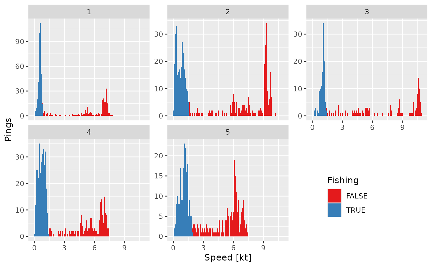
gg.base +
  geom_point(data = d,
             aes(time, speed, colour = Fishing),
             size = 0.5) +
  scale_colour_brewer(palette = "Set1") +
  labs(x = "Time", y = "Speed [kt]") +
  theme(legend.position = c(0.8, 0.2))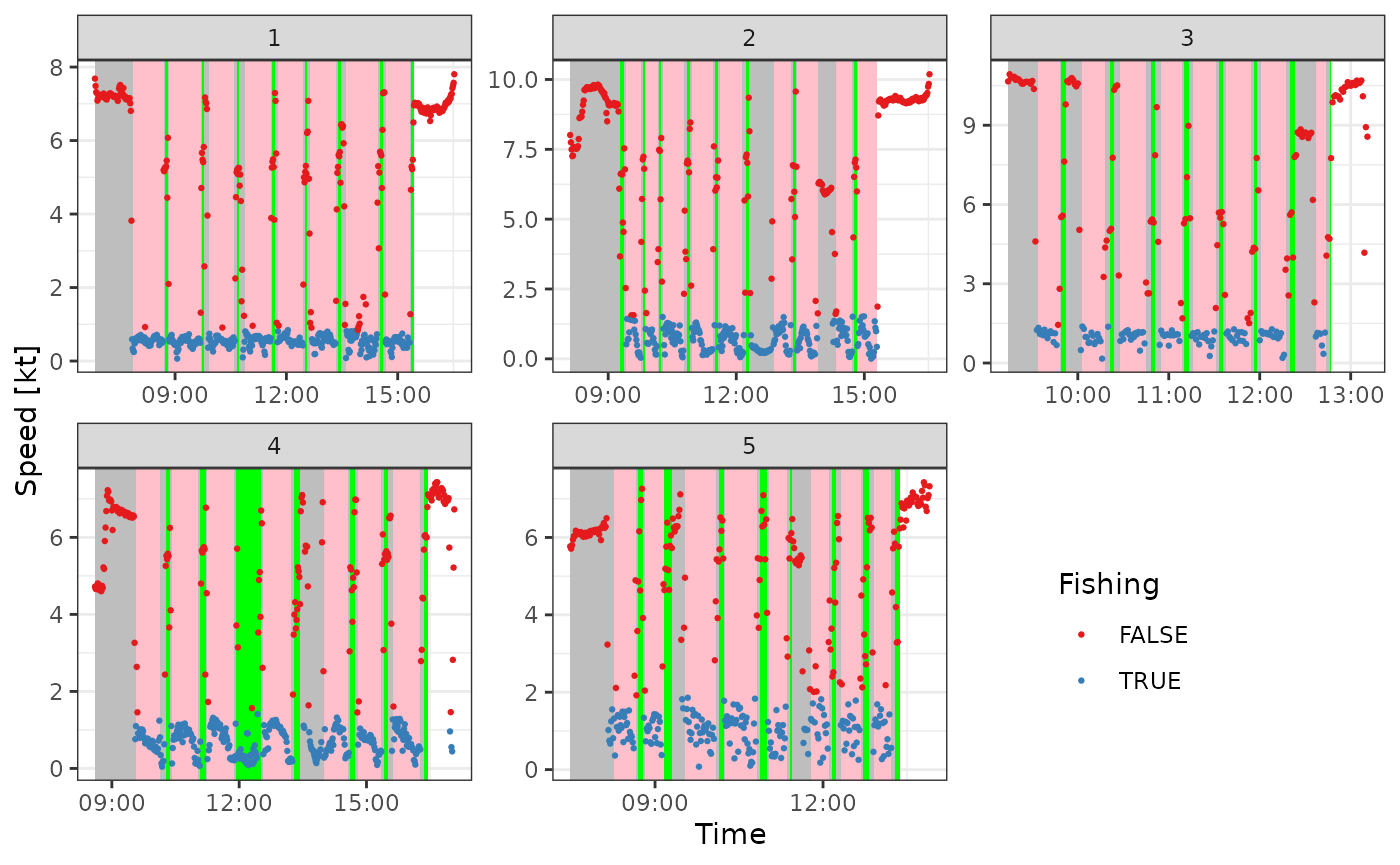
Model 3: Trip-based Binary Clustering using Gaussian mixture models on a trip-by-trip basis
d <-
  creel %>%
  group_by(id) %>%
  ramb::rb_gaussian_binary_clustering() %>%
  mutate(Fishing = ifelse(A %in% 1:2, TRUE, FALSE))
#> [1]   0  -0.0000e+00       4       583
#> [1] ... Stable clustering
#> [1]   0  -0.0000e+00       4       507
#> [1] ... Stable clustering
#> [1]   0  -0.0000e+00       4       239
#> [1] ... Stable clustering
#> [1]   0  -0.0000e+00       4       510
#> [1] ... Stable clustering
#> [1]   0  -0.0000e+00       4       387
#> [1] ... Stable clustering
d %>%
  count(behaviour, A) %>%
  spread(A, n) %>%
knitr::kable()| behaviour | 1 | 2 | 3 | 4 | 5 |
|---|---|---|---|---|---|
| hauling | 859 | 263 | NA | 21 | NA |
| shooting | 1 | 25 | 95 | 89 | NA |
| steaming | 76 | 59 | 574 | 159 | 5 |
| behaviour | FALSE | TRUE |
|---|---|---|
| hauling | 21 | 1122 |
| shooting | 184 | 26 |
| steaming | 738 | 135 |
d %>%
  ggplot(aes(speed, turn, colour = factor(A))) +
  theme_bw() +
  geom_point(size = 1) +
  facet_wrap(~ id) +
  scale_colour_brewer(palette = "Set1") +
  labs(x = "Speed [nm]", y = "Turn", colour = "clusters") +
  theme(legend.position = c(0.8, 0.25))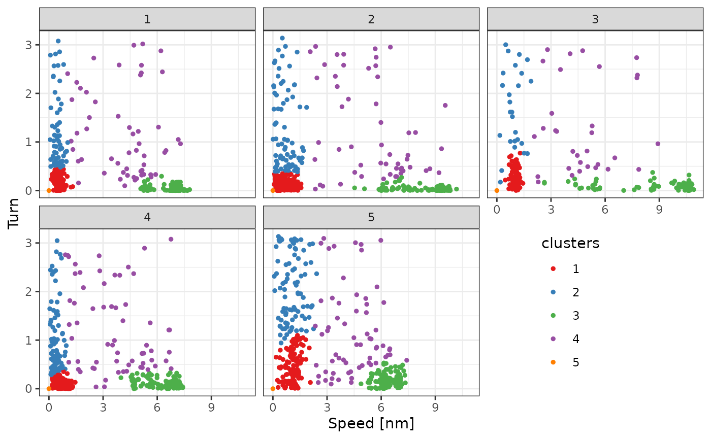
d %>%
  ggplot(aes(time, speed)) +
  theme_bw() +
  geom_point(aes(colour = factor(A)),
             size = 1) +
  facet_wrap(~ id, scales = "free") +
  theme(legend.position = c(0.8, 0.2)) +
  scale_colour_brewer(palette = "Set1") +
  labs(x = "Time", y = "Speed [kt]")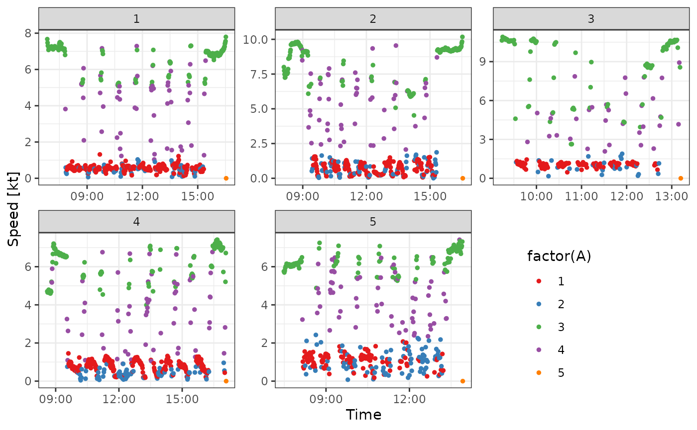
gg.base +
  geom_point(data = d,
             aes(time, speed, colour = Fishing),
             size = 0.5) +
  scale_colour_brewer(palette = "Set1") +
  labs(x = "Time", y = "Speed [kt]") +
  theme(legend.position = c(0.8, 0.2))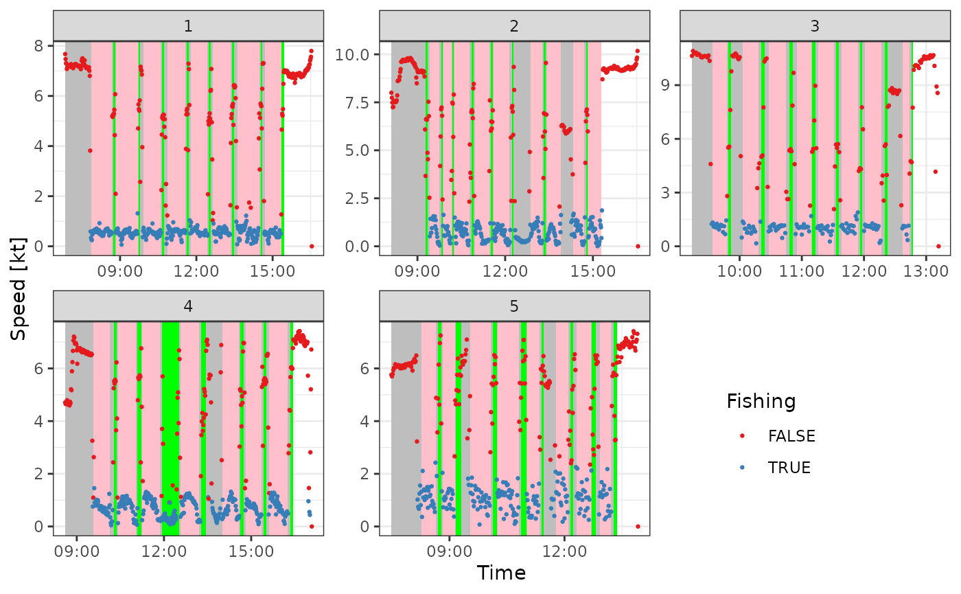
d %>%
  ggplot(aes(time, turn)) +
  theme_bw() +
  geom_point(aes(colour = factor(A)),
             size = 1) +
  facet_wrap(~ id, scales = "free") +
  theme(legend.position = c(0.8, 0.2)) +
  scale_colour_brewer(palette = "Set1") +
  labs(x = "Time", y = "Turn")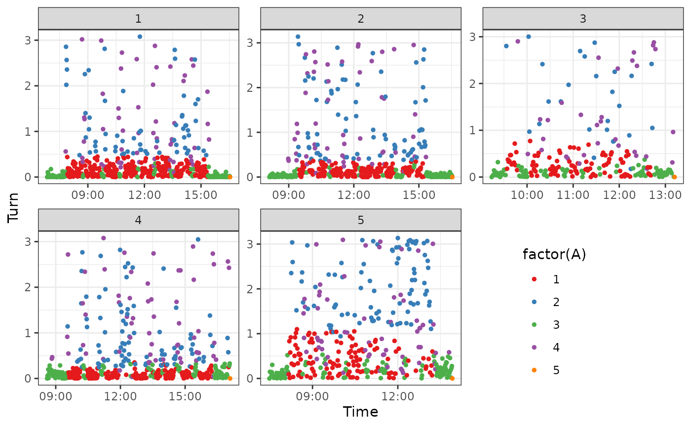
gg.base +
  geom_point(data = d,
             aes(time, turn, colour = Fishing),
             size = 0.5) +
  scale_colour_brewer(palette = "Set1") +
  labs(x = "Time", y = "Turn") +
  theme(legend.position = c(0.8, 0.2))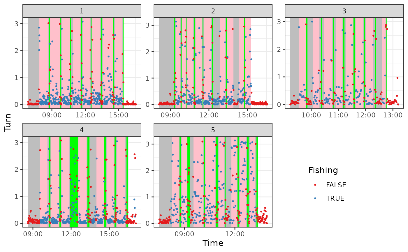
d %>%
  arrange(desc(A)) %>%
  ggplot(aes(lon, lat, colour = factor(A))) +
  theme_bw() +
  geom_point(size = 1) +
  facet_wrap(~ id, scales = "free") +
  coord_quickmap() +
  labs(x = NULL, y = NULL, colour = "clusters") +
  scale_colour_brewer(palette = "Set1") +
  theme(legend.position = c(0.8, 0.25))  +
  scale_x_continuous(NULL, NULL) +
  scale_y_continuous(NULL, NULL)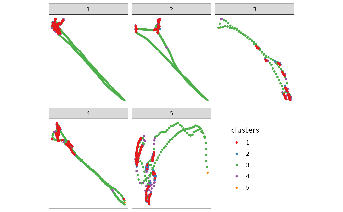
d %>%
  arrange(desc(A)) %>%
  ggplot(aes(lon, lat, colour = Fishing)) +
  theme_bw() +
  geom_point(size = 1) +
  facet_wrap(~ id, scales = "free") +
  coord_quickmap() +
  labs(colour = "Fishing") +
  scale_colour_brewer(palette = "Set1") +
  theme(legend.position = c(0.8, 0.25)) +
  scale_x_continuous(NULL, NULL) +
  scale_y_continuous(NULL, NULL)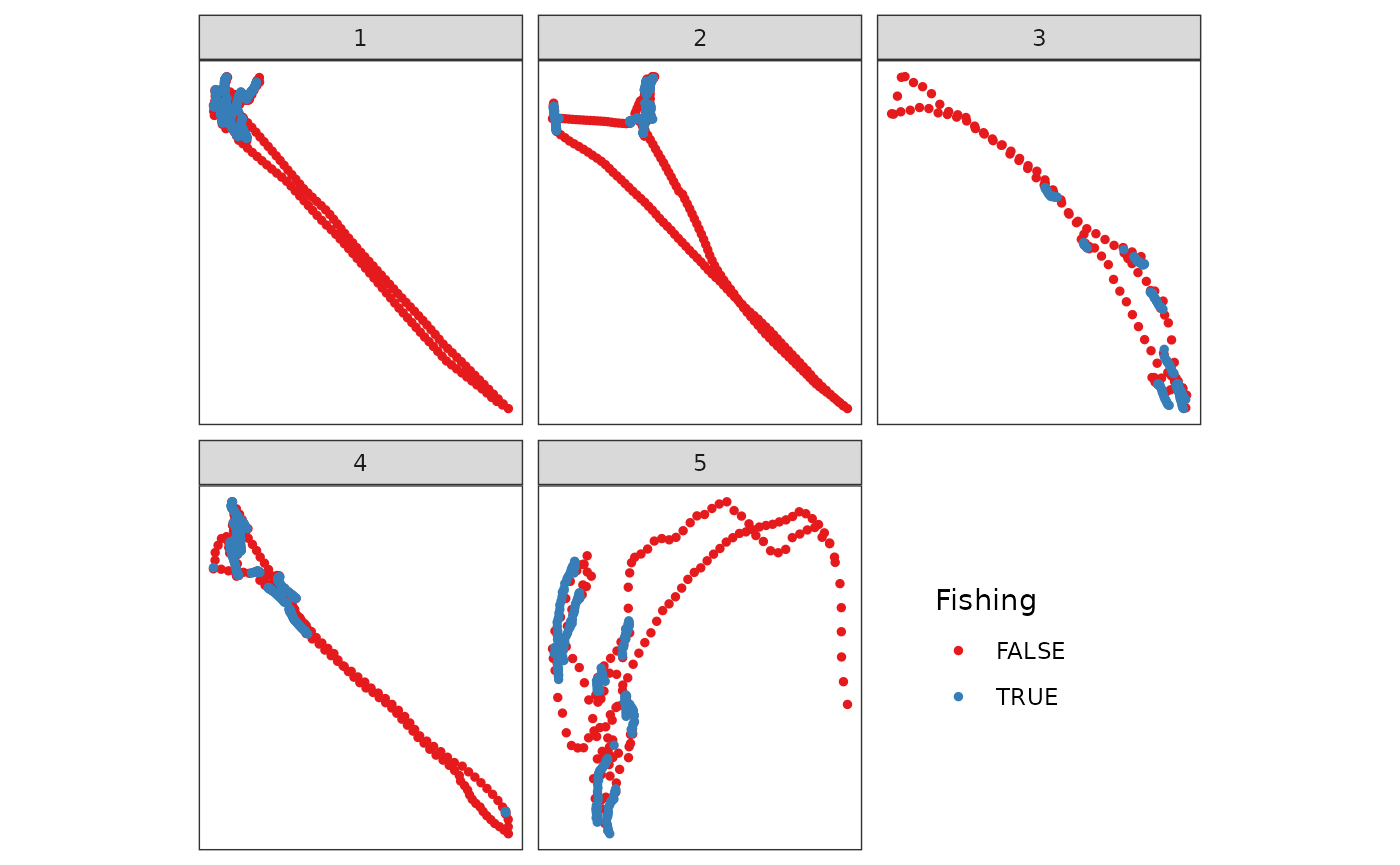
Model 4: Hidden Markov model with speed only
where is the speed here?
d <-
  creel %>%
  ramb::rb_hidden_markov_step()
#> number of iterations= 15
#> number of iterations= 19
#> number of iterations= 50
#> number of iterations= 20
#> number of iterations= 86
d %>%
  count(behaviour, vit) %>%
  spread(vit, n) %>%
knitr::kable()| behaviour | 1 | 2 | 3 |
|---|---|---|---|
| hauling | 1126 | 17 | NA |
| shooting | 29 | 155 | 26 |
| steaming | 147 | 234 | 487 |
gg.base +
  geom_point(data = d,
             aes(time, step, colour = factor(vit)),
             size = 0.5) +
  scale_colour_brewer(palette = "Set1") +
  labs(x = "Time", y = "Step [m]") +
  theme(legend.position = c(0.8, 0.2))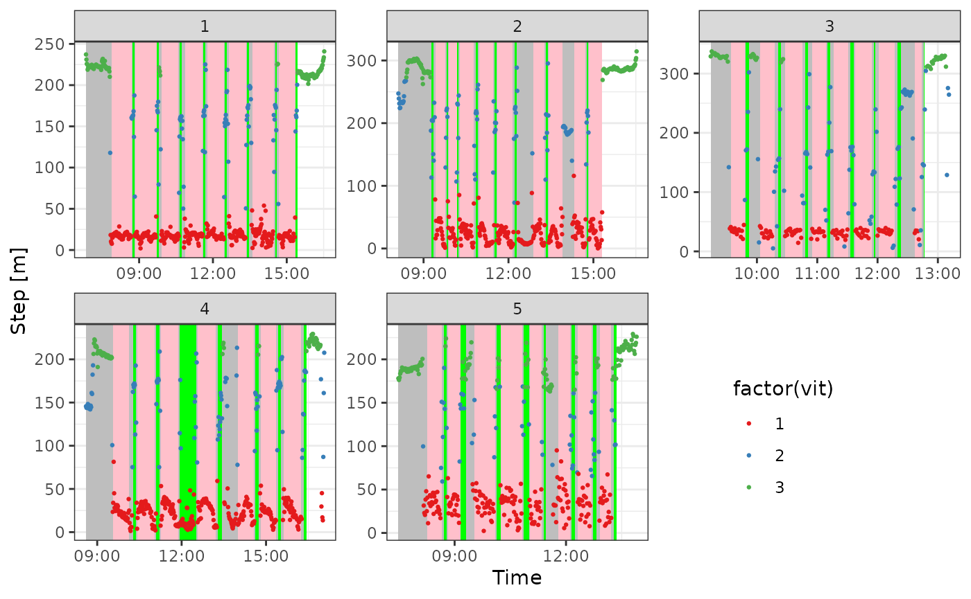
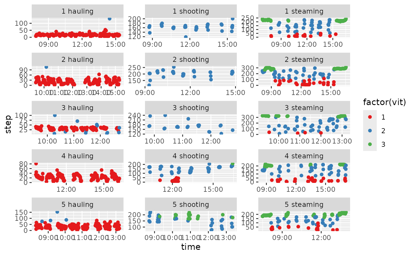
d %>%
  mutate(id = paste(id, behaviour)) %>%
  ggplot(aes(time, step, colour = factor(vit))) +
  geom_point() +
  facet_wrap(~id, scales = "free", ncol = 3) +
  scale_colour_brewer(palette = "Set1")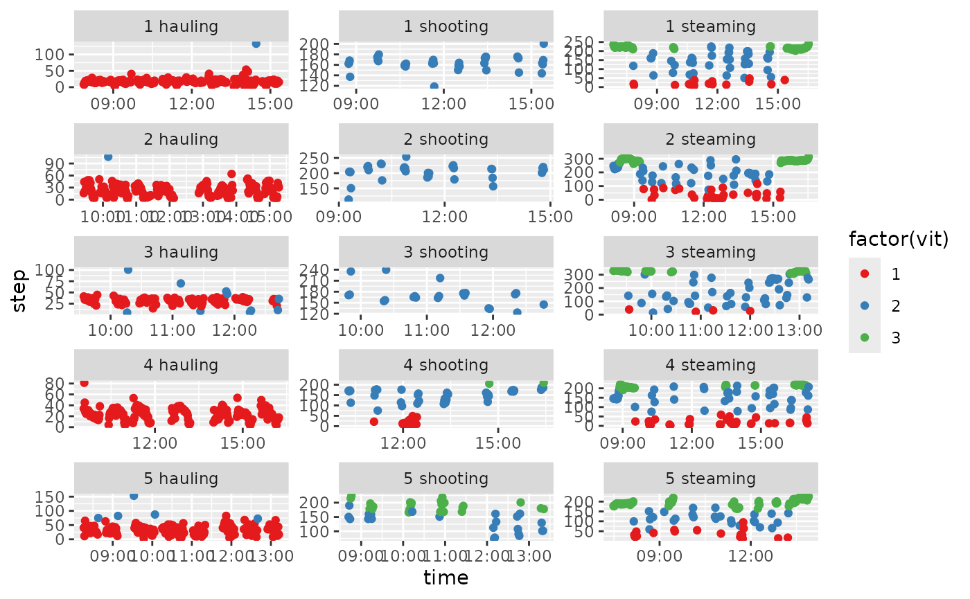
# why not on speed??Model 5: Hidden Markov Model with speed and turning angle
d <-
  creel %>%
  ramb::rb_hidden_markov_step_and_turn()
#> number of iterations= 16
#> number of iterations= 19
#> number of iterations= 50
#> number of iterations= 21
#> number of iterations= 85
gg.base +
  geom_point(data = d,
             aes(time, step, colour = factor(vit)),
             size = 0.5) +
  scale_colour_brewer(palette = "Set1") +
  labs(x = "Time", y = "Step [m]") +
  theme(legend.position = c(0.8, 0.2))
d %>%
  mutate(id = paste(id, behaviour)) %>%
  ggplot(aes(time, step, colour = factor(vit))) +
  geom_point() +
  facet_wrap(~id, scales = "free", ncol = 3) +
  scale_colour_brewer(palette = "Set1")