Transformation 2
Preamble
Commonly, when collating summaries by group, one wants to:
- Split up a big data structure into homogeneous pieces,
- Apply a function to each piece
- Combine all the results back together.
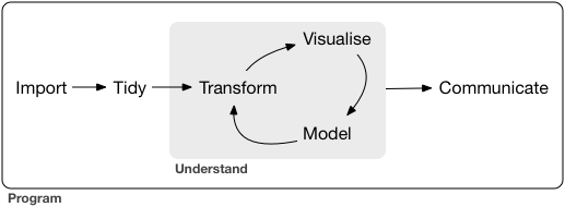
Reading material
Libraries and data
library(tidyverse)
w <- read_csv("https://heima.hafro.is/~einarhj/data/minke.csv")
Summarise cases
summarise:
To summarise data one uses the summarise-function. Below we calculate the number of observations (using the n-function and the mean minke length.
w |>
  summarise(n.obs = n(),
            ml = mean(length, na.rm = TRUE))
# A tibble: 1 × 2
n.obs ml
<int> <dbl>
1 190 753.group_by:
The power of the command summarise is revealed when used in conjunction with group_by-function. The latter functions splits the data into groups based on one or multiple variables. E.g. one can split the minke table by maturity:
w |>
  group_by(maturity)
# A tibble: 190 × 13
# Groups: maturity [6]
id date lon lat area length weight age sex
<dbl> <dttm> <dbl> <dbl> <chr> <dbl> <dbl> <dbl> <chr>
1 1 2004-06-10 22:00:00 -21.4 65.7 North 780 NA 11.3 Female
2 690 2004-06-15 17:00:00 -21.4 65.7 North 793 NA NA Female
3 926 2004-06-22 01:00:00 -19.8 66.5 North 858 NA 15.5 Female
4 1333 2003-09-30 16:00:00 -21.6 65.7 North 567 NA 7.2 Male
5 1334 2003-09-25 15:00:00 -15.6 66.3 North 774 NA 12.3 Female
6 1335 2003-09-16 16:00:00 -18.7 66.2 North 526 NA 9.6 Female
7 1336 2003-09-12 17:00:00 -21.5 65.7 North 809 NA 17.3 Female
8 1338 2003-09-09 12:00:00 -22.8 66.1 North 820 NA 13.8 Female
9 1339 2003-08-31 13:00:00 -17.5 66.6 North 697 NA 12.2 Male
10 1341 2003-08-30 17:00:00 -14.7 66.2 North 777 NA 15.4 Male
# ℹ 180 more rows
# ℹ 4 more variables: maturity <chr>, stomach.volume <dbl>,
# stomach.weight <dbl>, year <dbl>The table appears “intact” because it still has 190 observations but it has 6 groups, representing the different values of the maturity scaling in the data (anoestrous, immature, mature, pregnant, pubertal and “NA”).
The summarise-command respects the grouping, as shown if one uses the same command as used above, but now on a dataframe that has been grouped:
w |>
  group_by(maturity) |>
  summarise(n.obs = n(),
            mean = mean(length))
# A tibble: 6 × 3
maturity n.obs mean
<chr> <int> <dbl>
1 anoestrous 6 784.
2 immature 25 619.
3 mature 74 758.
4 pregnant 66 800.
5 pubertal 6 692.
6 <NA> 13 752.- Calculate the number of observations and minimum, median, mean, standard deviation and standard error of whale lengths in each year
- The function names in R are:
- n
- min
- max
- median
- mean
- sd
The function for standard error is not availble in R. A remedy is that you use college statistical knowledge to derive them from the appropriate variables you derived above.
This may help to find different basic statistics function.
w |>
  group_by(year) |>
  summarise(n = n(),
            min = min(length),
            max = max(length),
            median = median(length),
            mean = mean(length),
            sd = sd(length),
            se = sd / sqrt(n))
Note: If you would not be using the pipe-code-flow your code would be something like this:
summarise(group_by(w, year),
          n = n(),
          min = min(length))  # etc.
Shown because you are bound to come accross code like this.
Multiple group splitting
w |>
  group_by(maturity, year) |>
  summarise(n = n(),
            min = min(length),
            max = max(length),
            median = median(length),
            mean = mean(length),
            sd = sd(length),
            se = sd / sqrt(n),
            .groups = "drop") |>
knitr::kable(digits = 2)| maturity | year | n | min | max | median | mean | sd | se |
|---|---|---|---|---|---|---|---|---|
| anoestrous | 2004 | 1 | 819 | 819 | 819.0 | 819.00 | NA | NA |
| anoestrous | 2005 | 1 | 762 | 762 | 762.0 | 762.00 | NA | NA |
| anoestrous | 2006 | 4 | 761 | 804 | 780.5 | 781.50 | 17.60 | 8.80 |
| immature | 2003 | 6 | 508 | 774 | 534.0 | 572.83 | 100.64 | 41.09 |
| immature | 2004 | 3 | 502 | 712 | 684.0 | 632.67 | 114.02 | 65.83 |
| immature | 2005 | 8 | 474 | 737 | 640.5 | 624.12 | 109.84 | 38.84 |
| immature | 2006 | 4 | 461 | 706 | 604.5 | 594.00 | 100.76 | 50.38 |
| immature | 2007 | 4 | 622 | 760 | 695.5 | 693.25 | 56.82 | 28.41 |
| mature | 2003 | 17 | 693 | 845 | 771.0 | 765.88 | 35.40 | 8.59 |
| mature | 2004 | 10 | 685 | 836 | 771.0 | 764.10 | 47.20 | 14.93 |
| mature | 2005 | 13 | 566 | 870 | 740.0 | 743.85 | 72.19 | 20.02 |
| mature | 2006 | 24 | 606 | 857 | 750.5 | 750.50 | 59.67 | 12.18 |
| mature | 2007 | 10 | 701 | 819 | 792.5 | 777.10 | 39.35 | 12.44 |
| pregnant | 2003 | 9 | 730 | 861 | 809.0 | 801.00 | 39.88 | 13.29 |
| pregnant | 2004 | 10 | 745 | 858 | 814.0 | 809.10 | 42.88 | 13.56 |
| pregnant | 2005 | 7 | 752 | 871 | 825.0 | 822.29 | 44.59 | 16.85 |
| pregnant | 2006 | 19 | 732 | 858 | 802.0 | 799.26 | 38.42 | 8.81 |
| pregnant | 2007 | 21 | 682 | 871 | 790.0 | 787.00 | 49.71 | 10.85 |
| pubertal | 2003 | 3 | 603 | 697 | 692.0 | 664.00 | 52.89 | 30.53 |
| pubertal | 2005 | 1 | 764 | 764 | 764.0 | 764.00 | NA | NA |
| pubertal | 2006 | 2 | 692 | 706 | 699.0 | 699.00 | 9.90 | 7.00 |
| NA | 2003 | 1 | 840 | 840 | 840.0 | 840.00 | NA | NA |
| NA | 2004 | 1 | 634 | 634 | 634.0 | 634.00 | NA | NA |
| NA | 2005 | 4 | 740 | 790 | 775.0 | 770.00 | 24.49 | 12.25 |
| NA | 2006 | 5 | 662 | 803 | 763.0 | 745.60 | 53.44 | 23.90 |
| NA | 2007 | 2 | 716 | 780 | 748.0 | 748.00 | 45.25 | 32.00 |
Joins
Normally the data we are interested in working with do not reside in one table. E.g. for a typical survey data one stores a “station table” separate from a “detail” table. The surveys could be anything, e.g. catch sampling at a landing site or scientific trawl or UV-surveys.
Lets read in the Icelandic groundfish survey tables in such a format:
station <-
  read_csv("https://heima.hafro.is/~einarhj/data/is_smb_stations.csv")
biological <-
  read_csv("https://heima.hafro.is/~einarhj/data/is_smb_biological.csv")
station %>% select(id:lat1) %>%  arrange(id) %>% glimpse()
Rows: 19,846
Columns: 9
$ id <dbl> 29654, 29655, 29656, 29657, 29658, 29659, 29660, 29661, 29662, …
$ date <date> 1985-03-21, 1985-03-20, 1985-03-20, 1985-03-20, 1985-03-20, 19…
$ year <dbl> 1985, 1985, 1985, 1985, 1985, 1985, 1985, 1985, 1985, 1985, 198…
$ vid <dbl> 1273, 1273, 1273, 1273, 1273, 1273, 1273, 1273, 1273, 1273, 127…
$ tow_id <chr> "374-3", "374-11", "374-12", "373-13", "373-11", "373-12", "373…
$ t1 <dttm> 1985-03-21 00:45:00, 1985-03-20 22:25:00, 1985-03-20 20:35:00,…
$ t2 <dttm> 1985-03-21 01:50:00, 1985-03-20 23:25:00, 1985-03-20 21:45:00,…
$ lon1 <dbl> -24.17967, -24.19783, -24.40467, -23.99833, -23.67983, -23.7210…
$ lat1 <dbl> 63.96350, 63.75367, 63.71817, 63.58000, 63.74767, 63.83767, 63.…biological %>% arrange(id) %>% glimpse()Rows: 68,834
Columns: 4
$ id <dbl> 29654, 29654, 29654, 29654, 29655, 29655, 29655, 29655, 29656,…
$ species <chr> "cod", "haddock", "saithe", "wolffish", "cod", "haddock", "sai…
$ kg <dbl> 53.4895900, 29.6435494, 22.8682684, 0.6901652, 29.6210500, 203…
$ n <dbl> 13, 15, 5, 1, 6, 155, 23, 4, 6, 156, 39, 4, 43, 421, 8, 11, 25…Here the information on the station, such as date, geographical location are kept separate from the detail measurments that are performed at each station (weight and numbers by species). The records in the station table are unique (i.e. each station information only appear once) while we can have more than one species measured at each station. Take note here that the biological table does not contain records of species that were not observed at that station. The link between the two tables, in this case, is the variable id.
Take also note that there are 6 species in the data
biological |> count(species)# A tibble: 6 × 2
species n
<chr> <int>
1 cod 19425
2 haddock 16458
3 monkfish 2038
4 plaice 6388
5 saithe 8440
6 wolffish 16085but that the number of records by species is different between species. E.g. there are 19425 records of cod (out of 19846 stations) but only 2038 records of monkfish. Not storing zero records is quite common in databases. It is thus the responsibility of the user to understand the structure of the data and how to deal with zero’s vs. missing data (NA) in the downstream analysis.
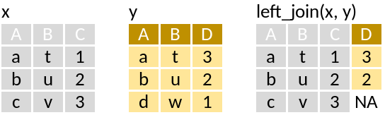
left_join: Matching values from y to x
Lets say we were interested in combining the geographical position and the species records from one station:
station %>%
  select(id, date, lon1, lat1) %>%
  filter(id == 29654) %>%
  left_join(biological)
# A tibble: 4 × 7
id date lon1 lat1 species kg n
<dbl> <date> <dbl> <dbl> <chr> <dbl> <dbl>
1 29654 1985-03-21 -24.2 64.0 cod 53.5 13
2 29654 1985-03-21 -24.2 64.0 haddock 29.6 15
3 29654 1985-03-21 -24.2 64.0 saithe 22.9 5
4 29654 1985-03-21 -24.2 64.0 wolffish 0.690 1Take note here:
- The joining is by common variable name in the two tables (here id)
- That we only have records of fours species in this table, again a value of zero for a species is not stored in the data.
If we were to want to obtain the records for monkfish from this survey we could do:
d <-
  station %>%
  select(id, date, lon1, lat1) |>
  left_join(biological |>
              filter(species == "monkfish"),
            by = join_by(id))
d
# A tibble: 19,846 × 7
id date lon1 lat1 species kg n
<dbl> <date> <dbl> <dbl> <chr> <dbl> <dbl>
1 44929 1990-03-16 -20.7 66.5 <NA> NA NA
2 44928 1990-03-16 -20.5 66.5 <NA> NA NA
3 44927 1990-03-16 -20.4 66.6 <NA> NA NA
4 44926 1990-03-16 -20.2 66.6 <NA> NA NA
5 44925 1990-03-16 -20.0 66.7 <NA> NA NA
6 44922 1990-03-16 -20.7 67.2 <NA> NA NA
7 44921 1990-03-16 -20.7 67.3 <NA> NA NA
8 44920 1990-03-17 -20.5 67.2 <NA> NA NA
9 44919 1990-03-17 -20.2 67.1 <NA> NA NA
10 44918 1990-03-17 -20.2 66.7 <NA> NA NA
# ℹ 19,836 more rowsNow we have 19846 records, but most of them have missing mass (kg) and abundance (n). To account for the zeros we would need to do the following additional steps:
d <-
  d |>
  mutate(species = replace_na(species, "monkfish"),
         kg = replace_na(kg, 0),
         n = replace_na(n, 0))
d
# A tibble: 19,846 × 7
id date lon1 lat1 species kg n
<dbl> <date> <dbl> <dbl> <chr> <dbl> <dbl>
1 44929 1990-03-16 -20.7 66.5 monkfish 0 0
2 44928 1990-03-16 -20.5 66.5 monkfish 0 0
3 44927 1990-03-16 -20.4 66.6 monkfish 0 0
4 44926 1990-03-16 -20.2 66.6 monkfish 0 0
5 44925 1990-03-16 -20.0 66.7 monkfish 0 0
6 44922 1990-03-16 -20.7 67.2 monkfish 0 0
7 44921 1990-03-16 -20.7 67.3 monkfish 0 0
8 44920 1990-03-17 -20.5 67.2 monkfish 0 0
9 44919 1990-03-17 -20.2 67.1 monkfish 0 0
10 44918 1990-03-17 -20.2 66.7 monkfish 0 0
# ℹ 19,836 more rowsSo only now would we able to do some summary statistics like the mean catch and standard error. Lets just use the inbuilt ggplot function to do that and get a plot at the same time:
d |>
  mutate(year = year(date)) |>
  ggplot(aes(year, kg)) +
  stat_summary(fun.data = "mean_cl_boot")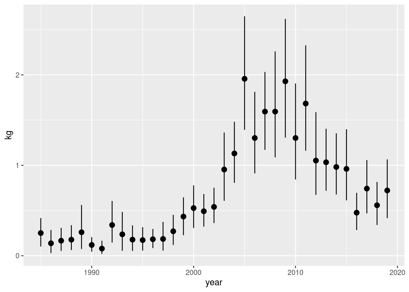
If we had done this without considering zero stations we have:
d |>
  mutate(year = year(date)) |>
  filter(kg != 0) |>
  ggplot(aes(year, kg)) +
  stat_summary(fun.data = "mean_cl_boot")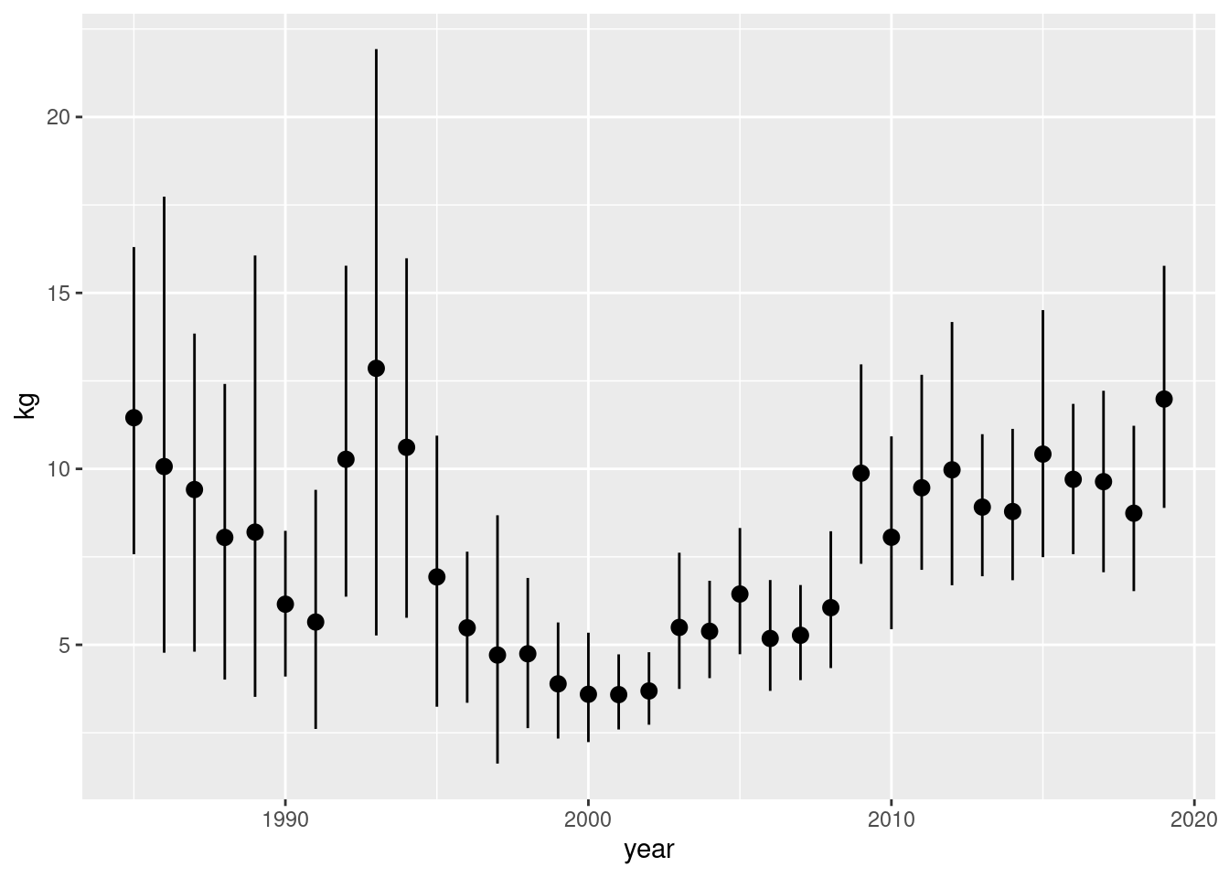
Ergo: When working with data in general it is always important to think about if missingness constitutes a zero or a true NA.
But we may want some tabular data, so we could do this rather than directly a plot:
d_sum <-
  d |>
  mutate(year = year(date)) |>
  group_by(year) |>
  summarise(n = n(),
            min_kg = min(kg),
            max_kg = max(kg),
            mean_kg = mean(kg),
            sd_kg = sd(kg),
            se_kg = sd_kg / sqrt(n),
            error = se_kg * 1.96,
            sum_kg = sum(kg))
d_sum
# A tibble: 35 × 9
year n min_kg max_kg mean_kg sd_kg se_kg error sum_kg
<dbl> <int> <dbl> <dbl> <dbl> <dbl> <dbl> <dbl> <dbl>
1 1985 593 0 31.5 0.251 2.04 0.0839 0.164 149.
2 1986 585 0 34.6 0.138 1.64 0.0678 0.133 80.5
3 1987 566 0 20.2 0.166 1.57 0.0661 0.130 94.1
4 1988 544 0 23.1 0.178 1.62 0.0696 0.136 96.6
5 1989 568 0 70.2 0.260 3.10 0.130 0.255 148.
6 1990 567 0 14.4 0.119 0.986 0.0414 0.0811 67.7
7 1991 570 0 18.3 0.0793 0.903 0.0378 0.0741 45.2
8 1992 574 0 53.5 0.340 2.76 0.115 0.226 195.
9 1993 597 0 48.7 0.237 2.67 0.109 0.214 141.
10 1994 596 0 24.4 0.178 1.72 0.0706 0.138 106.
# ℹ 25 more rowsAnd then the plot would be:
d_sum |>
  mutate(se_lower = mean_kg - error,
         se_upper = mean_kg + error) |>
  ggplot() +
  geom_pointrange(aes(year, mean_kg, ymin = se_lower, ymax = se_upper),
                  size = 0.5)
right_join: Matching values from x to y
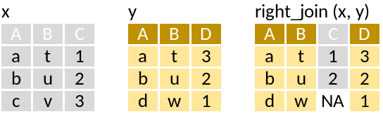
This is really the inverse of left_join.
inner_join: Retain only rows with matches
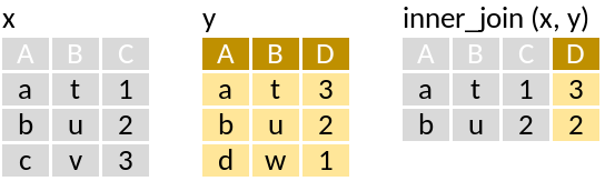
Example of only joining station information with monkfish, were monkfish was recorded:
station %>%
  inner_join(biological %>%
               filter(species == "monkfish"))
# A tibble: 2,038 × 31
id date year vid tow_id t1 t2
<dbl> <date> <dbl> <dbl> <chr> <dttm> <dttm>
1 44154 1990-03-11 1990 1273 374-1 1990-03-11 10:25:00 1990-03-11 11:30:00
2 44271 1990-03-12 1990 1273 323-1 1990-03-12 09:15:00 1990-03-12 10:25:00
3 44382 1990-03-13 1990 1273 320-4 1990-03-13 14:20:00 1990-03-13 15:20:00
4 44156 1990-03-11 1990 1273 374-3 1990-03-11 07:10:00 1990-03-11 08:15:00
5 44379 1990-03-14 1990 1273 320-3 1990-03-14 01:40:00 1990-03-14 02:40:00
6 44377 1990-03-14 1990 1273 320-12 1990-03-14 05:45:00 1990-03-14 06:50:00
7 44375 1990-03-14 1990 1273 321-11 1990-03-14 09:30:00 1990-03-14 10:40:00
8 44373 1990-03-14 1990 1273 371-12 1990-03-14 13:30:00 1990-03-14 14:20:00
9 44356 1990-03-16 1990 1273 366-11 1990-03-16 00:50:00 1990-03-16 01:30:00
10 50775 1992-03-15 1992 1273 371-12 1992-03-15 09:00:00 1992-03-15 10:10:00
# ℹ 2,028 more rows
# ℹ 24 more variables: lon1 <dbl>, lat1 <dbl>, lon2 <dbl>, lat2 <dbl>,
# ir <chr>, ir_lon <dbl>, ir_lat <dbl>, z1 <dbl>, z2 <dbl>, temp_s <dbl>,
# temp_b <dbl>, speed <dbl>, duration <dbl>, towlength <dbl>,
# horizontal <dbl>, verical <dbl>, wind <dbl>, wind_direction <dbl>,
# bormicon <dbl>, oldstrata <dbl>, newstrata <dbl>, species <chr>, kg <dbl>,
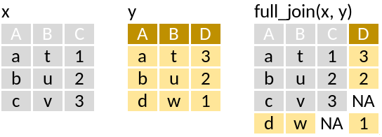
# n <dbl>full_join: Retain all rows
station %>%
  full_join(biological %>%
              filter(species == "monkfish")) %>%
  select(id, species:n)
# A tibble: 19,846 × 4
id species kg n
<dbl> <chr> <dbl> <dbl>
1 44929 <NA> NA NA
2 44928 <NA> NA NA
3 44927 <NA> NA NA
4 44926 <NA> NA NA
5 44925 <NA> NA NA
6 44922 <NA> NA NA
7 44921 <NA> NA NA
8 44920 <NA> NA NA
9 44919 <NA> NA NA
10 44918 <NA> NA NA
# ℹ 19,836 more rowsHere all the stations records are retained irrepsective if monkfish was caught or not.
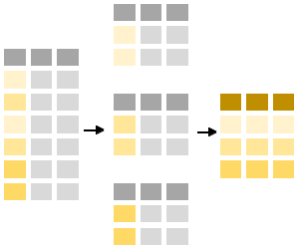
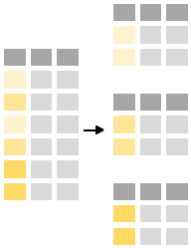
Run through this set of code that supposedly mimics the pictograms above:
x <- tibble(A = c("a", "b", "c"),
B = c("t", "u", "v"),
C = c(1, 2, 3))
y <- tibble(A = c("a", "b", "d"),
B = c("t", "u", "w"),
D = c(3, 2, 1))
x
y
left_join(x, y)
right_join(x, y)
left_join(y, x)
inner_join(x, y)
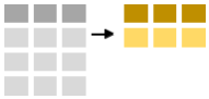
full_join(x, y)Combine cases (bind)
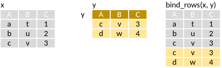
bind_rows: One on top of the other as a single table.
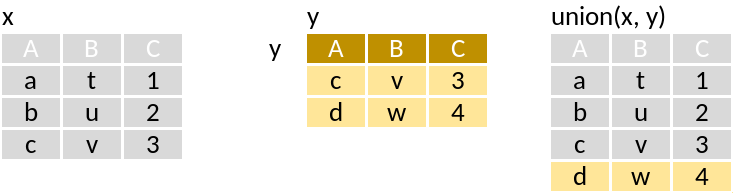
union: Rows in x or y
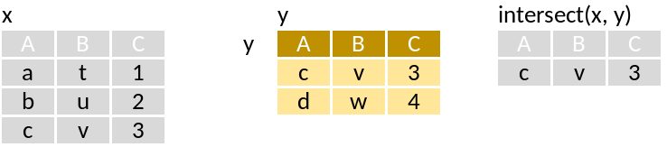
intersect: Rows in x and y.
setdiff: Rows in x but not y
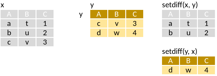
Run through this set of code that supposedly mimics the pictograms above:
x <- tibble(A = c("a", "b", "c"),
            B = c("t", "u", "v"),
            C = c(1, 2, 3))

y <- tibble(A = c("c", "d"),
            B = c("v", "w"),
            C = c(3, 4))
x
y
bind_rows(x, y)
union(x, y)
intersect(x, y)
setdiff(x, y)
setdiff(y, x)