Quering MFRI databases

Preamble

To access the MFRI database you need:

The {ROracle} package (which needs the {DBI} package)
The {mar} package

Testing if you have {ROracle} and {mar} installed:

system.file(package = "ROracle")

[1] "/home/haf/einarhj/R/x86_64-pc-linux-gnu-library/4.3/ROracle"

system.file(package = "mar")

[1] "/home/haf/einarhj/R/x86_64-pc-linux-gnu-library/4.3/mar"

Ideally these should be installed by the IT-department when they set up your computer, including R and RStudio.

Installing {ROracle}

If you do not have ROracle do:

pth <- "https://r.hafro.is/bin/windows/contrib/4.2/ROracle_1.3-1.1.zip"
download.file(pth, destfile = "ROracle_1.3-1.1.zip")
install.packages("ROracle_1.3-1.1.zip", repos = NULL, type = "win.binary")
file.remove("ROracle_1.3-1.1.zip")

Installing {mar}

If you do not have mar do:

remotes::install_git(
  "https://gitlab.hafogvatn.is/dev/mar.git", 
  dependencies = FALSE)

Connecting to the database

library(tidyverse)
library(mar)
con <- connect_mar()
con

User name:             ops$einarhj 
Connect string:        sjor 
Server version:        19.0.0.0.0 
Server type:           Oracle RDBMS 
Results processed:     0 
OCI prefetch:          FALSE 
Bulk read:             1000 
Bulk write:            1000 
Statement cache size:  0 
Open results:          0

What is in the database?

The mar_tables-function gives us some informations about what is in the database:

info <- mar_tables(con)
info |> glimpse()

Rows: ??
Columns: 6
Database: OraConnection
$ owner           <chr> "sys", "sys", "sys", "sys", "sys", "sys", "sys", "sys"…
$ table_name      <chr> "dual", "system_privilege_map", "table_privilege_map",…
$ comments        <chr> NA, "Description table for privilege type codes.  Maps…
$ tablespace_name <chr> "SYSTEM", "SYSTEM", "SYSTEM", "SYSTEM", "SYSTEM", NA, …
$ num_rows        <dbl> 1, 257, 26, 4, 337, NA, NA, 1, 239, 457, 0, NA, NA, NA…
$ last_analyzed   <dttm> 2023-06-23 22:00:59, 2021-04-30 22:00:37, 2021-04-26 …

Here we have among other things:

owner: This is sometimes referred to as “schema”. Basically a schema contains a number of tables that may or may not be related. Let’s count the number of table.
table_name: An actual table.
comments: Hopefully some useful description of what is in the table.

What schemas do we have?

Let’s see the schemas we have and how many tables in each schema:

info |> 
  count(owner, name = "n.tables") |> 
  arrange(owner) |> 
  collect() |> 
  knitr::kable(caption = "List of owners and the number of tables")

List of owners and the number of tables
owner	n.tables
adb	15
afli	19
agf	3
asfis	1
ask	9
ata	28
bathymetry	1
biota	35
botndyr	27
channel	35
ctxsys	5
erfdafraedi	8
fiskar	4
fiskifelagid	2
fiskmerki	21
flokkun	14
fuglar	8
gear	18
hafmynd	26
hafro	10
hafvog	3
hvalir	2
hydro	40
kvoti	19
mdsys	57
merki	24
nyting	3
ops\(anika \| 7\| \|ops\)bthe	46
ops\(einarhj \| 51\| \|ops\)ella	3
ops\(krik \| 2\| \|ops\)mdan	1
ops\(pamela \| 8\| \|ops\)rafn	3
ops\(sigfus \| 4\| \|ops\)will	9
orri	9
pame	1
phyto	13
selir	14
siritar	5
stk	13
svifthorungar	17
syni	15
sys	45
system	41
taxon	7
telogger	2
thorungar	15
ufs	2
veidibok	10
vessel	18
worms	1
xdb	6

What tables do we have?

Let’s check what tables are in phyto:

info |> 
  filter(owner == "phyto") |> 
  select(table_name, comments) |> 
  arrange(table_name) |> 
  collect()

# A tibble: 13 × 2
   table_name  comments                                                         
   <chr>       <chr>                                                            
 1 dypi        "Í töflunni eru upplýsingar ýmissa umhverfisþátta, sem hafa veri…
 2 hafur       "Í töflunni eru upplýsingar um hvaða þörungategundir hafa fundis…
 3 observation  <NA>                                                            
 4 prod        "Tafla eftir eyðslu á dálkunum year og turner"                   
 5 prod_old    "Gögn eftir eyðslu á year og the_date > '83 gögnum"              
 6 stadur      "Í töflunni eru upplýsingar um staðarnöfn þar sem mælingar hafa\…
 7 station      <NA>                                                            
 8 station_old  <NA>                                                            
 9 stodvar     "Í töflunni eru upplýsingar um stað og stund þar sem sýnataka fe…
10 talning     "Í töflunni eru upplýsingar um fjölda einstaklinga af tiltekinni…
11 tegundir    "Í töflunni er ein færsla fyrir hverja þörungategund. Ýmiss kona…
12 tmp_obs      <NA>                                                            
13 underway     <NA>

What views do we have?

Because the construct of tables within a database can be quite complex, a view is often created that may combine different tables. The intent is to make it easier for the downstream user to operate on the data. Let’s check what views are in veidibok:

mar_views(con) |> 
  filter(owner == "veidibok") |> 
  arrange(view_name) |> 
  collect() |> 
  knitr::kable()

owner	view_name
veidibok	fisktegundir_v
veidibok	notendur_v
veidibok	vbs_vf_dagveidi_v
veidibok	vbs_vf_fjoldi_kyn_heiti_v
veidibok	vbs_vf_fjoldi_kyn_v
veidibok	vbs_vf_fjoldi_tegund_heiti_v
veidibok	vbs_vf_fjoldi_tegund_v
veidibok	vbs_vf_lengdardreif_heiti_v
veidibok	vbs_vf_lengdardreifing_v
veidibok	vbs_vf_stadur_veidi_heiti_v
veidibok	vbs_vf_stadur_veidi_v
veidibok	vbs_vf_thyngdardreif_heiti_v
veidibok	vbs_vf_thyngdardreifing_v
veidibok	vbs_vf_thyngdardreif_kyn_v
veidibok	vbs_vf_thyngdardr_kyn_heiti_v
veidibok	vbs_vf_thyngdartolur_v
veidibok	vbs_vf_thyngd_heiti_v
veidibok	vbs_vf_vikuveidi_heiti_v
veidibok	vbs_vf_vikuveidi_v
veidibok	vbs_vs_dagveidi_v
veidibok	vbs_vs_fjoldi_kyn_heiti_v
veidibok	vbs_vs_fjoldi_kyn_v
veidibok	vbs_vs_fjoldi_tegund_heiti_v
veidibok	vbs_vs_fjoldi_tegund_v
veidibok	vbs_vs_lengdardreif_heiti_v
veidibok	vbs_vs_lengdardreifing_v
veidibok	vbs_vs_stadur_veidi_heiti_v
veidibok	vbs_vs_stadur_veidi_v
veidibok	vbs_vs_thyngdardreif_heiti_v
veidibok	vbs_vs_thyngdardreifing_v
veidibok	vbs_vs_thyngdardreif_kyn_v
veidibok	vbs_vs_thyngdardr_kyn_heiti_v
veidibok	vbs_vs_thyngdartolur_v
veidibok	vbs_vs_thyngd_heiti_v
veidibok	vbs_vs_vikuveidi_heiti_v
veidibok	vbs_vs_vikuveidi_v
veidibok	veidibok_v
veidibok	veidi_samtals_v
veidibok	veidi_v

What variables are in a table?

Here we use the mar_fields-function. Lets pick the table “phyto.hafur”

mar_fields(con, "phyto.talning")

# Source:   SQL [?? x 4]
# Database: OraConnection
   owner table_name column_name comments                                        
   <chr> <chr>      <chr>       <chr>                                           
 1 phyto talning    snt         <NA>                                            
 2 phyto talning    snn         <NA>                                            
 3 phyto talning    sbt         <NA>                                            
 4 phyto talning    sbn         <NA>                                            
 5 phyto talning    s_id        Númer sem tengir færsluna við ákveðna stöð, lyk…
 6 phyto talning    dypi        <NA>                                            
 7 phyto talning    skst        Skammstöfun tegundarinnar, lykill í TEGUNDIR.   
 8 phyto talning    fjoldi      Fjöldi fruma á líter.                           
 9 phyto talning    dags_taln   Dagsetning talningar.                           
10 phyto talning    rummal      Rúmmál talningarhólks í ml.                     
# ℹ more rows

What is in a table?

Here we use the function tbl_mar:

tbl_mar(con, "fiskmerki.rafgogn")

# Source:   SQL [?? x 6]
# Database: OraConnection
        id taudkenni    nr dagstimi             dypi hitastig
     <dbl> <chr>     <dbl> <dttm>              <dbl>    <dbl>
 1 8299166 1C1426     6362 2004-06-13 17:30:00  171.     3.34
 2 8299167 1C1426     6363 2004-06-13 17:40:00  168.     3.34
 3 6763843 2C0669    43559 2005-02-11 03:00:00  212.     6.35
 4 8299168 1C1426     6364 2004-06-13 17:50:00  169.     3.34
 5 8299169 1C1426     6365 2004-06-13 18:00:00  168.     3.34
 6 6763846 2C0669    43560 2005-02-11 03:10:00  214.     6.35
 7 8299170 1C1426     6366 2004-06-13 18:10:00  168.     3.34
 8 8299171 1C1426     6367 2004-06-13 18:20:00  168.     3.38
 9 6763849 2C0669    43561 2005-02-11 03:20:00  213.     6.35
10 8299172 1C1426     6368 2004-06-13 18:30:00  168.     3.38
# ℹ more rows

Exercise: Take a look at a table of your own choice

Use the mar_tables-, mar_views-, mar_fields, tbl_mar-functions to explore something of your interest
If you do not have read access to certain schemas/tables but you think you should, send an email to Rafn Sigurðsson at hafogvatn.is

Under the hood

The basic function when we access a database table is tbl. Let’s use to explain what is happening under the hood, here taking a peek at a simple “lookup-table”:

q <- tbl(con, dbplyr::in_schema("VESSEL", "USAGE_CATEGORY"))
q |> glimpse()

Rows: ??
Columns: 5
Database: OraConnection
$ USAGE_CATEGORY_NO <int> 231, 154, 6299, 6283, 6252, 6237, 6289, 46, 50, 55, …
$ CODE              <dbl> 116, 115, 129, 118, NA, 117, 132, 201, 202, 203, 204…
$ NAME              <chr> "A - FARÞEGASKIP", "A - FLUTNINGASKIP", "A - FLUTNIN…
$ ENG_NAME          <chr> "PASSENGER SHIP", "CARGO SHIP", "Other cargo ship", …
$ CATEGORY          <chr> "OtherShip", "OtherShip", "OtherShip", "OtherShip", …

Take note here that:

We do not get the number of rows
That it is stated “Database: OraConnection”
Look into your “Environment” as see that q i actually “List of 2”, not the usual “x obs. of y variables”

So we have kind of a table but not quite the tables we have so far worked with in R. Check out this e.g.:

q |> class()

[1] "tbl_OraConnection" "tbl_dbi"           "tbl_sql"          
[4] "tbl_lazy"          "tbl"

q |> show_query()

<SQL>
SELECT *
FROM "VESSEL"."USAGE_CATEGORY"

Effectively what we have is an SQL-query. Let’s add a filter:

q2 <- 
  q |> 
  filter(CATEGORY == "FishingShip") |> 
  select(name = NAME, english = ENG_NAME, cat = CATEGORY)
q2 |> glimpse()

Rows: ??
Columns: 3
Database: OraConnection
$ name    <chr> "FISKISKIP", "FRÍSTUNDAFISKISKIP", "HVALVEIÐISKIP", "NÓTAVEIÐI…
$ english <chr> "FISHING VESSEL", NA, NA, NA, "Research Vessel", "TRAWLER", NA
$ cat     <chr> "FishingShip", "FishingShip", "FishingShip", "FishingShip", "F…

q2 |> show_query()

<SQL>
SELECT "NAME" AS "name", "ENG_NAME" AS "english", "CATEGORY" AS "cat"
FROM "VESSEL"."USAGE_CATEGORY"
WHERE ("CATEGORY" = 'FishingShip')

So now we have more SQL-code. The big news here is:

We can use the R-functions we already have learned
Because we are communicating with a database the R-code is converted into SQL-code automatically
Now Oracle only “understands” SQL. But we do not need to learn that language because the dbplyr-package does that for us. Consider yourself blessed.

Note though that not every code in R is translated to SQL

Normally we would not access a table by the tbl-function, user rather the tbl_mar-function, e.g.:

q <- tbl_mar(con, "vessel.usage_category")
q |> glimpse()

Rows: ??
Columns: 5
Database: OraConnection
$ usage_category_no <int> 231, 154, 6299, 6283, 6252, 6237, 6289, 46, 50, 55, …
$ code              <dbl> 116, 115, 129, 118, NA, 117, 132, 201, 202, 203, 204…
$ name              <chr> "A - FARÞEGASKIP", "A - FLUTNINGASKIP", "A - FLUTNIN…
$ eng_name          <chr> "PASSENGER SHIP", "CARGO SHIP", "Other cargo ship", …
$ category          <chr> "OtherShip", "OtherShip", "OtherShip", "OtherShip", …

Sometimes there is a shortcut available, like:

q <- taggart(con)
q |> glimpse()

Rows: ??
Columns: 37
Database: OraConnection
$ fiskur_id    <dbl> 56255, 56256, 56257, 56258, 56259, 56260, 56261, 56262, 5…
$ synis_id     <dbl> 236952, 236952, 236952, 236952, 236952, 236952, 236952, 2…
$ tTegund      <dbl> 23, 23, 23, 23, 23, 23, 23, 23, 23, 23, 23, 23, 23, 23, 2…
$ tLengd       <dbl> 39, 39, 38, 32, 42, 40, 36, 42, 49, 47, 31, 50, 35, 40, 3…
$ tThyngd      <dbl> 0, 0, 0, 0, 0, 0, 0, 0, 0, 0, 0, 0, 0, 0, 0, 0, 0, 0, 0, …
$ tKyn         <dbl> NA, NA, NA, NA, NA, NA, NA, NA, NA, NA, NA, NA, NA, NA, N…
$ tKynthroski  <dbl> NA, NA, NA, NA, NA, NA, NA, NA, NA, NA, NA, NA, NA, NA, N…
$ audkenni     <chr> "IH", "IH", "IH", "IH", "IH", "IH", "IH", "IH", "IH", "IH…
$ numer        <dbl> 1122, 1775, 1634, 1316, 1565, 1137, 1656, 1830, 1922, 110…
$ leidangur    <chr> "B3-73", "B3-73", "B3-73", "B3-73", "B3-73", "B3-73", "B3…
$ stod         <dbl> 1424, 1424, 1424, 1424, 1424, 1424, 1424, 1424, 1424, 142…
$ tDags        <dttm> 1973-03-07, 1973-03-07, 1973-03-07, 1973-03-07, 1973-03-…
$ tAr          <dbl> 1973, 1973, 1973, 1973, 1973, 1973, 1973, 1973, 1973, 197…
$ tReitur      <dbl> 422, 422, 422, 422, 422, 422, 422, 422, 422, 422, 422, 42…
$ tSmareitur   <dbl> 3, 3, 3, 3, 3, 3, 3, 3, 3, 3, 3, 3, 3, 3, 3, 3, 3, 3, 3, …
$ tLon         <dbl> -22.95, -22.95, -22.95, -22.95, -22.95, -22.95, -22.95, -…
$ tLat         <dbl> 64, 64, 64, 64, 64, 64, 64, 64, 64, 64, 64, 64, 64, 64, 6…
$ tDypi        <dbl> 95, 95, 95, 95, 95, 95, 95, 95, 95, 95, 95, 95, 95, 95, 9…
$ tVeidarfaeri <dbl> 7, 7, 7, 7, 7, 7, 7, 7, 7, 7, 7, 7, 7, 7, 7, 7, 7, 7, 7, …
$ rid          <dbl> NA, NA, NA, NA, NA, NA, NA, NA, NA, NA, NA, NA, NA, NA, N…
$ rDags        <dttm> NA, NA, NA, NA, NA, NA, NA, NA, NA, NA, NA, NA, NA, NA, …
$ rAr          <int> NA, NA, NA, NA, NA, NA, NA, NA, NA, NA, NA, NA, NA, NA, N…
$ rManudur     <int> NA, NA, NA, NA, NA, NA, NA, NA, NA, NA, NA, NA, NA, NA, N…
$ rLon         <dbl> NA, NA, NA, NA, NA, NA, NA, NA, NA, NA, NA, NA, NA, NA, N…
$ rLat         <dbl> NA, NA, NA, NA, NA, NA, NA, NA, NA, NA, NA, NA, NA, NA, N…
$ rReitur      <int> NA, NA, NA, NA, NA, NA, NA, NA, NA, NA, NA, NA, NA, NA, N…
$ rSmareitur   <int> NA, NA, NA, NA, NA, NA, NA, NA, NA, NA, NA, NA, NA, NA, N…
$ rLandshluti  <dbl> NA, NA, NA, NA, NA, NA, NA, NA, NA, NA, NA, NA, NA, NA, N…
$ rHafsvaedi   <dbl> NA, NA, NA, NA, NA, NA, NA, NA, NA, NA, NA, NA, NA, NA, N…
$ rVeidarfaeri <dbl> NA, NA, NA, NA, NA, NA, NA, NA, NA, NA, NA, NA, NA, NA, N…
$ rDypi        <dbl> NA, NA, NA, NA, NA, NA, NA, NA, NA, NA, NA, NA, NA, NA, N…
$ rTegund      <dbl> NA, NA, NA, NA, NA, NA, NA, NA, NA, NA, NA, NA, NA, NA, N…
$ rLengd       <dbl> NA, NA, NA, NA, NA, NA, NA, NA, NA, NA, NA, NA, NA, NA, N…
$ rKyn         <dbl> NA, NA, NA, NA, NA, NA, NA, NA, NA, NA, NA, NA, NA, NA, N…
$ rKynthroski  <dbl> NA, NA, NA, NA, NA, NA, NA, NA, NA, NA, NA, NA, NA, NA, N…
$ rAge         <dbl> NA, NA, NA, NA, NA, NA, NA, NA, NA, NA, NA, NA, NA, NA, N…
$ dst_id       <chr> NA, NA, NA, NA, NA, NA, NA, NA, NA, NA, NA, NA, NA, NA, N…

q |> show_query()

<SQL>
SELECT
  "FISKAR"."ID" AS "fiskur_id",
  "FISKAR"."SYNIS_ID" AS "synis_id",
  "TEGUND" AS "tTegund",
  "LENGD" AS "tLengd",
  "THYNGD" AS "tThyngd",
  "KYN" AS "tKyn",
  "KYNTHROSKI" AS "tKynthroski",
  "AUDKENNI" AS "audkenni",
  "NUMER" AS "numer",
  "leidangur",
  "stod",
  "tDags",
  "tAr",
  "tReitur",
  "tSmareitur",
  "tLon",
  "tLat",
  "tDypi",
  "tVeidarfaeri",
  "rid",
  "rDags",
  "rAr",
  "rManudur",
  "rLon",
  "rLat",
  "rReitur",
  "rSmareitur",
  "rLandshluti",
  "rHafsvaedi",
  "rVeidarfaeri",
  "rDypi",
  "rTegund",
  "rLengd",
  "rKyn",
  "rKynthroski",
  "rAge",
  "TAUDKENNI" AS "dst_id"
FROM "FISKMERKI"."FISKAR"
LEFT JOIN "FISKMERKI"."MERKI"
  ON ("FISKAR"."ID" = "MERKI"."FISKUR_ID")
LEFT JOIN (
  SELECT
    "SYNIS_ID" AS "synis_id",
    "LEIDANGUR" AS "leidangur",
    "STOD_V"."STOD_ID" AS "stod",
    "DAGS" AS "tDags",
    "AR" AS "tAr",
    "REITUR" AS "tReitur",
    "SMAREITUR" AS "tSmareitur",
    "KASTAD_LENGD" AS "tLon",
    "KASTAD_BREIDD" AS "tLat",
    "BOTNDYPI_KASTAD" AS "tDypi",
    "VEIDARFAERI" AS "tVeidarfaeri"
  FROM "CHANNEL"."STOD_V"
  LEFT JOIN "CHANNEL"."SYNI_V"
    ON ("STOD_V"."STOD_ID" = "SYNI_V"."STOD_ID")
) "...3"
  ON ("FISKAR"."SYNIS_ID" = "...3"."synis_id")
LEFT JOIN (
  SELECT
    "rid",
    "tid",
    "rDags",
    "rAr",
    "rManudur",
    -geoconvert1("rLon" * 100.0) AS "rLon",
    geoconvert1("rLat" * 100.0) AS "rLat",
    "rReitur",
    "rSmareitur",
    "rLandshluti",
    "rHafsvaedi",
    "rVeidarfaeri",
    "rDypi",
    "rTegund",
    "rLengd",
    "rKyn",
    "rKynthroski",
    "rAge"
  FROM (
    SELECT
      "ID" AS "rid",
      "MERKI_ID" AS "tid",
      "DAGS_FUNDID" AS "rDags",
      "AR" AS "rAr",
      "MANUDUR" AS "rManudur",
      "VLENGD" AS "rLon",
      "NBREIDD" AS "rLat",
      "REITUR" AS "rReitur",
      "SMAREITUR" AS "rSmareitur",
      "LANDSHLUTI_ID" AS "rLandshluti",
      "HAFSVAEDI_ID" AS "rHafsvaedi",
      "VEIDARFAERI_ID" AS "rVeidarfaeri",
      "DYPI" AS "rDypi",
      "TEGUND" AS "rTegund",
      "LENGD" AS "rLengd",
      "KYN" AS "rKyn",
      "KYNTHROSKI" AS "rKynthroski",
      "ALDUR" AS "rAge"
    FROM "FISKMERKI"."ENDURHEIMTUR"
  ) "q01"
) "...4"
  ON ("MERKI"."ID" = "...4"."tid")
LEFT JOIN "FISKMERKI"."RAFAUDKENNI"
  ON ("MERKI"."ID" = "RAFAUDKENNI"."MERKI_ID")

In both cases take note that the variable names now are all in small-caps (they are originally all-caps in Oracle).

Some “random” data view

Number of fish sampling stations

les_stod(con) |> 
  filter(between(ar, 1800, 2100)) |> 
  count(ar) |> 
  collect() |> 
  ggplot(aes(ar, n)) +
  geom_col() +
  labs(title = "Number of fish sampling stations")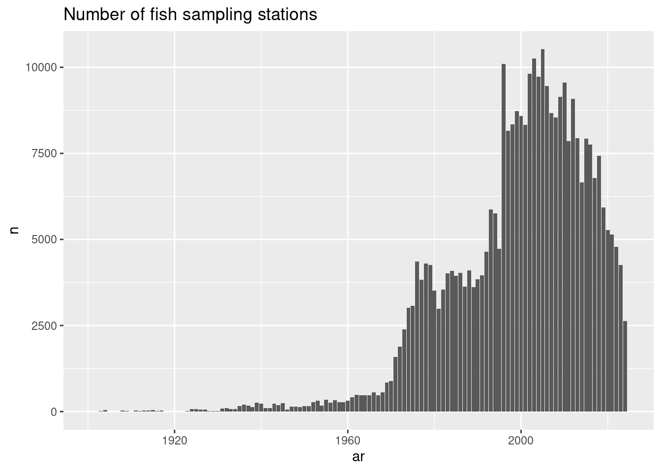

Electronic fish tag

q <- 
  tbl_mar(con, "fiskmerki.rafgogn") |> 
  filter(taudkenni == "1C0407")
q |> glimpse()

Rows: ??
Columns: 6
Database: OraConnection
$ id        <dbl> 8641662, 8641663, 8641664, 8641665, 8641666, 8641667, 864166…
$ taudkenni <chr> "1C0407", "1C0407", "1C0407", "1C0407", "1C0407", "1C0407", …
$ nr        <dbl> 1, 2, 3, 4, 5, 6, 7, 8, 9, 10, 11, 12, 13, 14, 15, 16, 17, 1…
$ dagstimi  <dttm> 2003-04-15 00:00:00, 2003-04-15 00:10:00, 2003-04-15 00:20:…
$ dypi      <dbl> 15.44, 15.44, 15.67, 15.44, 15.67, 15.67, 15.67, 15.67, 15.9…
$ hitastig  <dbl> 7.59, 7.59, 7.59, 7.59, 7.59, 7.59, 7.59, 7.59, 7.59, 7.59, …

q |> 
  collect() |> 
  ggplot(aes(dagstimi, -dypi)) +
  geom_point(size = 0.1) +
  labs(title = "Depth profile from one electronically tagged fish")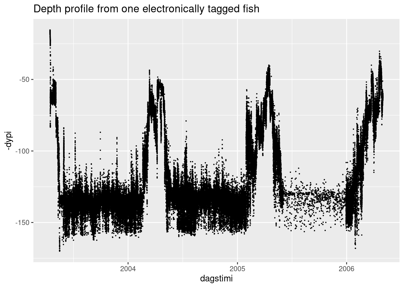

Hydro sonda

q <- 
  tbl_mar(con, "hydro.v_sonda") |> 
  filter(between(latitude, 66, 67),
         between(longitude, -19, -18))
q |> glimpse()

Rows: ??
Columns: 9
Database: OraConnection
$ l_id        <chr> "B6-89", "B6-89", "B6-89", "B6-89", "B6-89", "B6-89", "B6-…
$ id          <int> 479, 479, 479, 479, 479, 479, 479, 479, 479, 479, 479, 479…
$ datetime    <chr> "30.08.1989 12:00", "30.08.1989 12:00", "30.08.1989 12:00"…
$ latitude    <dbl> 66.4, 66.4, 66.4, 66.4, 66.4, 66.4, 66.4, 66.4, 66.4, 66.4…
$ longitude   <dbl> -18.8333, -18.8333, -18.8333, -18.8333, -18.8333, -18.8333…
$ pressure    <dbl> 1, 2, 3, 4, 5, 6, 7, 8, 9, 10, 11, 12, 13, 14, 15, 16, 17,…
$ temperature <dbl> 7.16, 7.16, 7.16, 7.16, 7.16, 7.13, 7.13, 7.13, 7.14, 7.14…
$ salinity    <dbl> 33.160, 33.173, 33.153, 33.152, 33.142, 33.146, 33.144, 33…
$ name        <chr> "SI2", "SI2", "SI2", "SI2", "SI2", "SI2", "SI2", "SI2", "S…

q |> 
  collect() |>  
  ggplot(aes(temperature, -pressure)) +
  theme_bw() +
  geom_point(size = 0.1, alpha = 0.05) +
  labs(title = "Temperature profiles")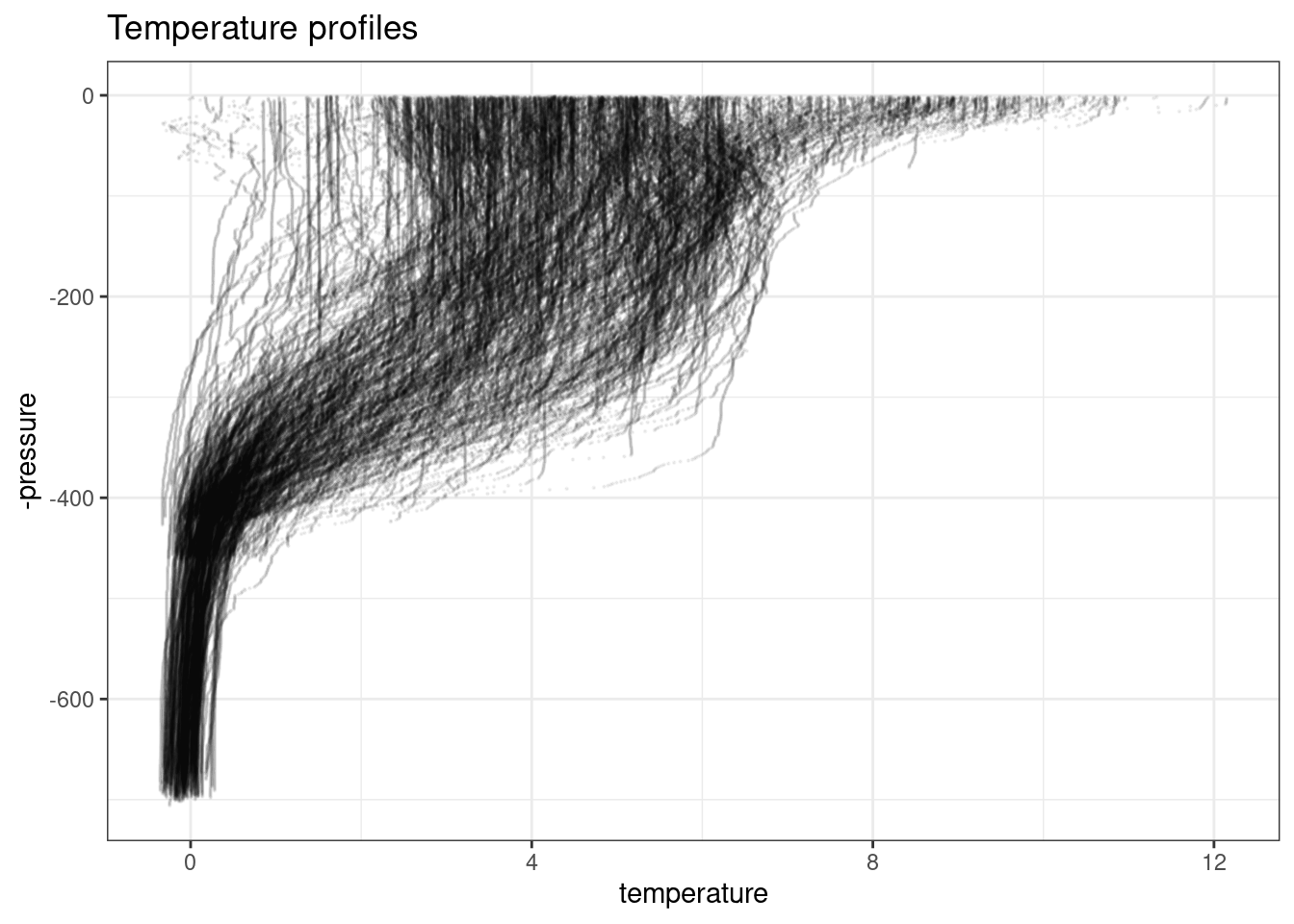

q |> 
  filter(between(pressure, 150, 200)) |> 
  mutate(year = str_sub(datetime, 7, 10),
         year = as.integer(year)) |> 
  ggplot(aes(year, temperature)) +
  stat_summary(fun.data = "mean_cl_boot") +
  labs(title = "Temperature change at pressure 150-200")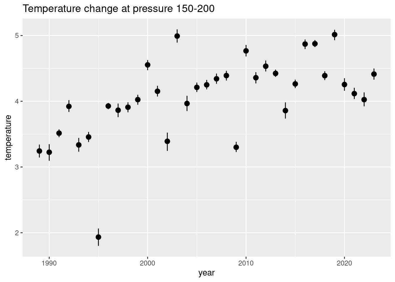

Veiðibók

tbl_mar(con, "veidibok.veidibok_v") |>
  filter(vatnsfall %in% 
           c("Laxá í Aðaldal", "Laxá á Ásum,", "Vatnsdalsá", "Ytri Rangá", 
             "Víðidalsá og Fitjá", "Eystri Rangá", "Norðurá Borg", "Apavatn",
             "Langá", "Hlíðarvatn", "Arnarvatn stóra", "Grímsá Borgarfirði",
             "Miðfjarðará", "Blanda", "Laxá í Kjós", "Hofsá í Vopnafirði",
             "Selá í Vopnafirði", "Fljótaá", "Eyjafjarðará", "Grenlækur")) |> 
  mutate(year = year(dags)) |> 
  count(year, vatnsfall, fisktegund) |> 
  collect() |> 
  ggplot(aes(year, n, fill = fisktegund)) +
  geom_col() +
  facet_wrap(~ vatnsfall, scales = "free_y", ncol = 2) +
  scale_fill_brewer(palette = "Set1") +
  labs(title = "Fjöldi fiska??")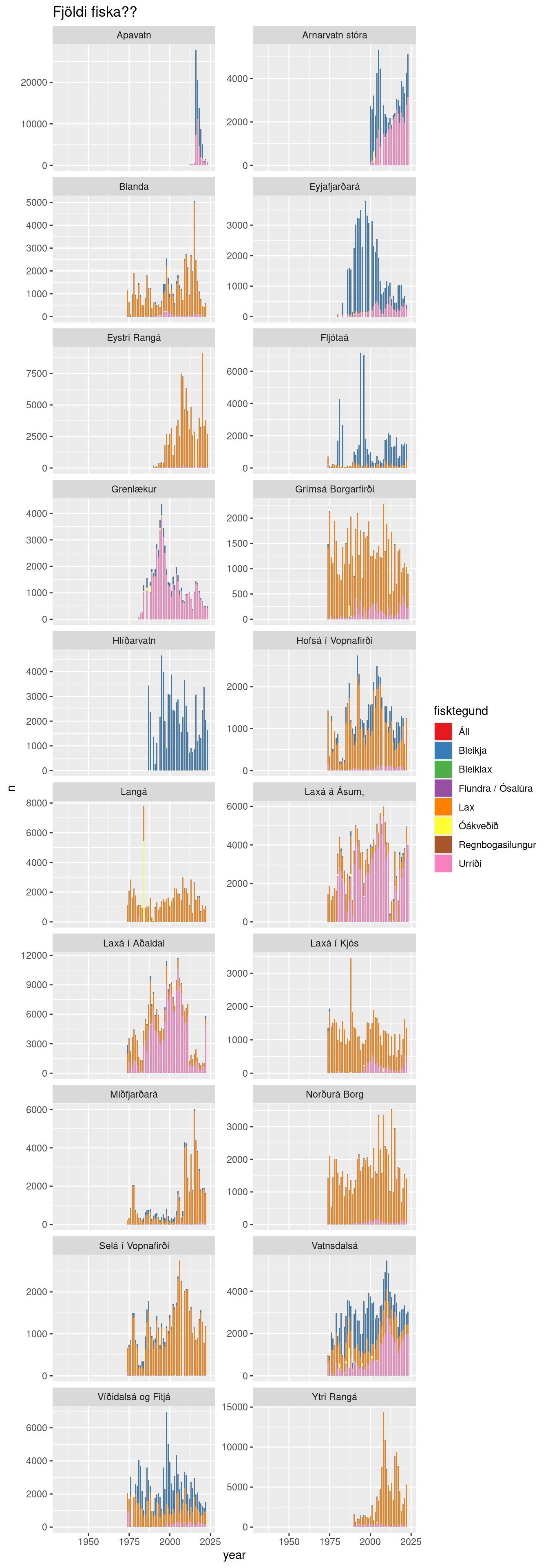

Exercise

Let’s collectively pick a table and look at some of the data
Try out yourself, but take note that you may not have read-access to only but few of the schemas and tables

Very complex R code

The following shows you can generate very complex query from within R. Here we connect to different tables and then join them using only R-syntax. This is actually the code behind the taggart-funtion used above.

stodvar <-
  les_stod(con) %>%
  left_join(les_syni(con), by = 'stod_id') %>% 
  # dplyr::mutate(tLon = kastad_lengd,
  #        tLat =  kastad_breidd,
  #        tAr = to_number(to_char(dags, 'yyyy'))) %>%
  dplyr::select(synis_id,
                leidangur,
                stod = stod_id,
                tDags = dags,
                tAr = ar,
                tReitur = reitur,
                tSmareitur = smareitur,
                tLon = kastad_lengd,
                tLat = kastad_breidd,
                tDypi = botndypi_kastad,
                tVeidarfaeri = veidarfaeri)

fiskar <-
  fiskmerki_fiskar(con) %>%
  dplyr::select(fiskur_id,
                synis_id,
                tTegund = tegund,
                tLengd = lengd,
                tThyngd = thyngd,
                tKyn = kyn,
                tKynthroski = kynthroski)

merki <-
  fiskmerki_merki(con) %>%
  dplyr::select(tid,
                fiskur_id,
                audkenni,
                numer)

q <-
  fiskar %>%
  dplyr::left_join(merki, by = "fiskur_id") %>%
  dplyr::left_join(stodvar, by = "synis_id") %>%
  dplyr::left_join(fiskmerki_endurheimtur(con), by = "tid") %>%
  dplyr::left_join(fiskmerki_rafaudkenni(con),  by = "tid") %>%
  dplyr::select(-id, -tid)

q |> show_query()