Haddock

Some of the main characteristics are

1.

Simulation period is from 1978 to 1999. Four timesteps are used each year

2.

The ages used are 1 to 10 years. The oldest age was treated as a plus group but with very high value of M.

3.

Survey indices were disaggregated in 5 cm length groups except for the smallest fish, where the length group size was chosen so all age 1 haddock ended in one length group.

4.

4 different alternatives were tested. Alternatives 1 and 2 use fixed growth but alternatives 3 and 4 estimate growth for each year after 1988. In alternatives 2 and 4 more weight was put on survey indices and less on catch data than in alternatives 1 and 3.

5.

Natural mortality was set to 0.5 for age 1, 0.35 for age 2, 0.2 for ages 3 to 7, 0.3 for age 8, 0.4 for age 9 and 0.7 for age 10.

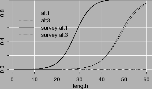
Here alternatives 1 and 3 will be those investigated. Figure 5.1 shows the estimated selection patterns and figure 5.2 the estimated recruitment. Selection patterns are similar for both alternatives while recruitment in recent years is usually better according to alternative 3. (growth is less)

  

Figure 5.1: Selection patterns of catch and survey

  

Figure 5.2: Estimated recruitment at age 1 accoring to the model

Figure 5.3 shows mean length at age according to alternative 1, excluding all length dependent mortality.

In alternatives 3 and 4 growth was estimated for every year with some penalty on changes between adjacent years. ($L_{\inf}$ in von Bertalanffys model was always the same). The factor that multiplies growth in weight is shown in table 5. It indicates that since 1989 growth in weight has been 5-15% less than before. Growth was of course variable before 1989 so the interannual variability of growth should be extended further back.

  

Figure 5.3: Estimated growth according to alternative 1

 

Table 5.1: Estimated multiplier for growth in weight

year	<89	89	90	91	92	93	94	95	96	>=97
mult	1.00	0.85	0.92	0.94	0.94	0.85	0.81	0.91	0.91	0.85

 

Future simulations were done with recruitment at age 1 after 1999 set to 90 million individuals, which is below long time average according to the model. In alternative 3 the growth multiplier was set to 0.9 after 1998. The following figures show development of catch, catchable biomass, and fishing mortality of age 7, using F = 0.4 0.6 0.8 1 1.2 1.4 and 1.6 for fish fully recruited to the catch. The estimated selection pattern indicates that only really large haddock > 50-60 cm are fully recruited to the catch (figure 5.1).

Figures 5.4 to 5.7 show development of catch, catchable biomass and fishing mortality of age 7 haddock. Alternative 1 where growth is fixed indicates higher fishing mortality today than alternative 3 does. This is logical as in alternative 1 (fixed growth) the only way for the model to get reduced weight at age is to increase fishing mortality. For management purposes the results in alternatives 1 and 3 are though similar, as less growth as in alternative 3 will give lower values of F_0.1 and F_max. Looking at figur 5.2 10% more recruitment should have been used in alternative 3 than in alternative 1.

  

Figure 5.4: Catch of haddock according to alternative 1.

  

Figure 5.5: Catchable biomass of haddock according to alternative 1

  

Figure 5.6: Fishing mortality of age 7 haddock according to alternative 1

  

Figure 5.7: Catch of haddock according to alternative 3.

  

Figure 5.8: Catchable biomass of haddock according to alternative 3

  

Figure 5.9: Fishing mortality of age 7 haddock according to alternative 3

Figure 5.10 shows estimated yield per recruit according to altenative 1. F_max is 0.5 and F_0.1 0.32. Less growth will give lower values of F_max and F_0.1.

Figures 5.11 to 5.13 show then the catchable biomass, catch and fishing mortality of age 7 haddock using F = 0.5 after 1998.

  

Figure 5.10: Estimated yield per recruit for haddock

  

Figure 5.11: Catch of haddock according to alternatives 1 and 3 (dotted line)

  

Figure 5.12: Catchable biomass of haddock according to alternative 1 and 3 (dotted line)

  

Figure 5.13: Fishing mortality of age 7 haddock according to alternatives 1 and 3 (dotted line)

5 shows the contribution of the objective function. Length distribution from the survey contribute 5% of the total objective function. It is possible that larger haddock is less available to the survey. In that case using logistic function as the selection curve for the survey could lead to overestimate of the mortality of larger haddock. The estimation done in alternative 3 was repeated without using length distributions in the survey, giving identical results.

Interesting aspect of table 5 is that mean length at age in survey and catch fit better in alternative 1 than in alternative 3 which is opposite to what would be expected.

 

Table 5.2: Distribution of the objective function on different components

tmp	alt1	%alt1	alt3	%alt3
Understocking	0.00	0.00	0.00	0.00
Alkeys catch	149040.00	15.70	142620.00	15.68
Alkeys survey	75640.00	7.97	75580.00	8.31
Bounds	0.00	0.00	0.00	0.00
Length distr catch	297300.00	31.31	276900.00	30.44
Length distr survey	46775.00	4.93	50750.00	5.58
Mean length catch	73575.00	7.75	80445.00	8.84
Mean length survey	26380.00	2.78	37100.00	4.08
Penalty on growth change			5595.00	0.62
Survey indices 8-22 cm	7413.00	0.78	6141.00	0.68
Survey indices 23-47 cm	171150.00	18.03	144990.00	15.94
Survey indices 48-62 cm	79960.00	8.42	68560.00	7.54
Survey indices 65-75 cm	22220.00	2.34	21010.00	2.31

 

In the original run with haddock all survey indices were in 5cm length group which split age 1 in 3 parts. This did not change much except in the estimate of the 1998 yearclass which was 30% higher in number. The reason for that was that it the mean length was less than average so unusually many fishes were between 7 and 12cm. The model then used that length group to lift the recruitment up but only the 1990 yearclass had comparable number of fishes so small.

Some additional work is planned on the haddock example.

1.

Use age disaggregated survey indices and compare to the solution using length disaggregated indices

2.

Try to incorporate an autumn survey that was started in 1994

3.

extend variability in growth further back