The Visual Raster Cheat Sheet

Etienne B. Racine (etiennebr@gmail.com)

2023-08-20 (R version 4.2.2 and raster package version 3.6.23)

Source code and package available at https://github.com/etiennebr/visualraster. Suggestions, contributions, feature request, and bug report are appreciated and help to keep that project alive.

I/O

Input and output operations, load or write data

raster

r = raster(matrix(sample(1:9, 100, replace = TRUE), 10, 10))

write

writeRaster(r, "raster.tif")

read

r = raster("raster.tif")

Local

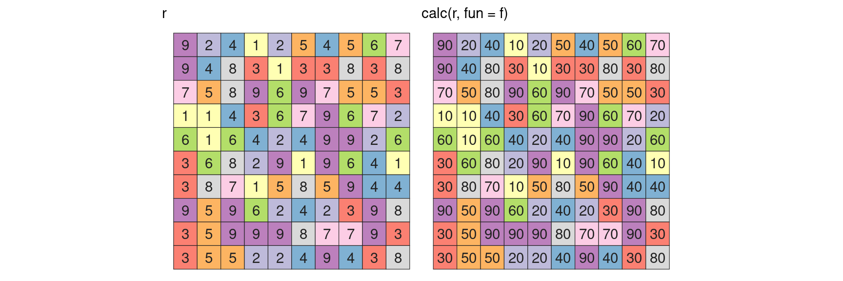
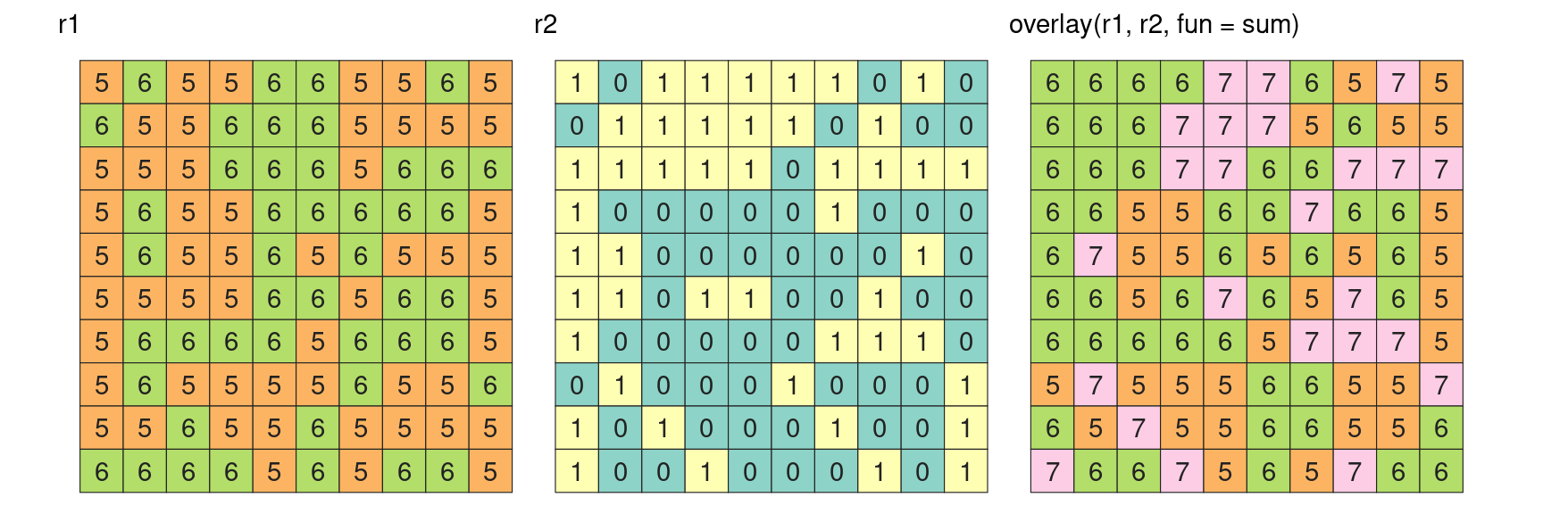
Local analysis consider cells independently

Access

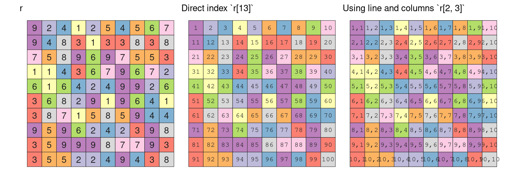
r[13]
#> [1] 8
r[2, 3]
#> [1] 8
r[2,  ]
#>  [1] 9 4 8 3 1 3 3 8 3 8
r[ , 3]
#>  [1] 4 8 8 4 6 8 7 9 9 5
#r[2:3, , drop = FALSE] |> lh()

Add vectors

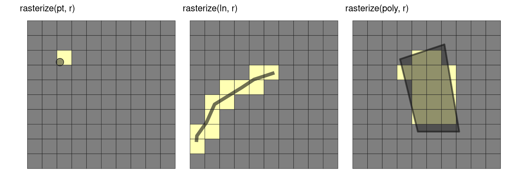
Cell from point

cellFromXY(r, pt)
#> [1] 23
colFromX(r, pt$x)
#> [1] 3
rowFromY(r, pt$y)
#> [1] 3
fourCellsFromXY(r, as.matrix(pt))
#>      [,1] [,2] [,3] [,4]
#> [1,]   23   33   32   22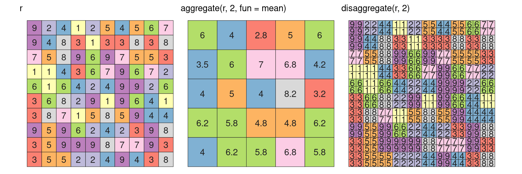

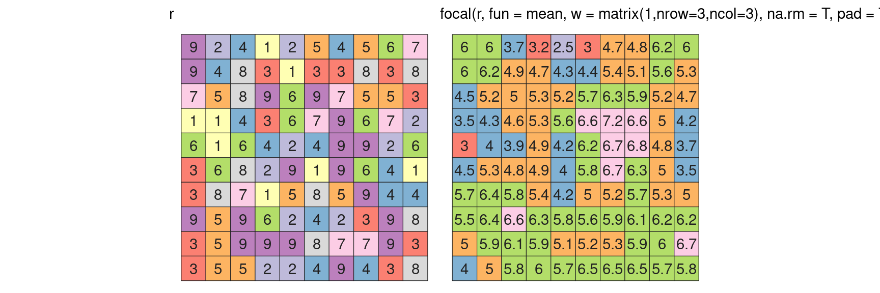
Cell from line

cellFromLine(r, ln)
#> [[1]]
#>  [1] 35 36 43 44 45 52 53 62 71 72 81

Cell from polygon

cellFromPolygon(r, poly)
#> [[1]]
#>  [1] 25 26 34 35 36 37 45 46 47 55 56 57 65 66 67

aggregate - disaggregate

cover

mask

calc

f = function(x) { x * 10 }

overlay

distance

We need a raster containing origins to compute distances (so we need units)

r_origin = raster(matrix(NA, 10, 10))
extent(r_origin) = extent(c(0, 10, 0, 10))
projection(r_origin) = "+proj=tmerc +lat_0=0 +lon_0=0 +x_0=0 +y_0=0 +units=m"
r_origin[c(15, 16, 45)] = 0

reclassify

m = cbind(
  from    = c(0, 2, 4), 
  to      = c(2, 4, 8), 
  becomes = c(1, 2, 3)
)

from	to	becomes
0	2	1
2	4	2
4	8	3

Focal

Focal analysis consider a cell plus its direct neighbours in a contiguous and symetrical manner

focal

r_focal = focal(r, fun = mean, w = matrix(1,nrow=3,ncol=3))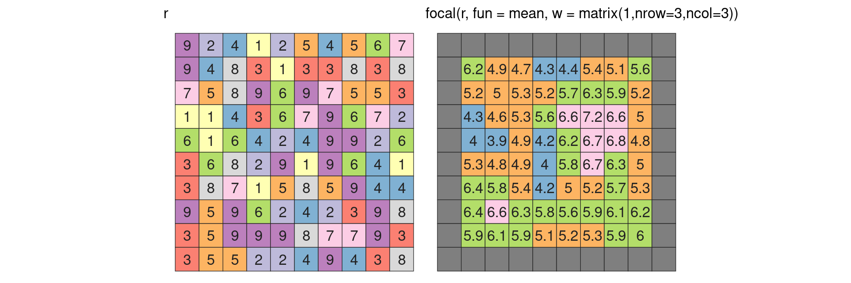

One can remove edge effect by ignoring NA values

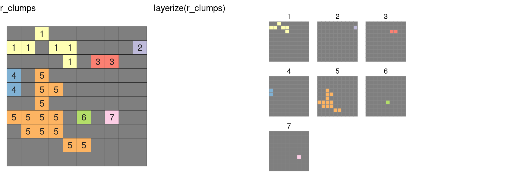
Zonal

Zonal analysis consider group of cells in an irregular, but conitguous (in space or value) manner.

zonal

QUO VADIS?

zonal(r, z, mean)

zone	value
0	2.0
1	5.3
2	5.6
3	5.2

clump

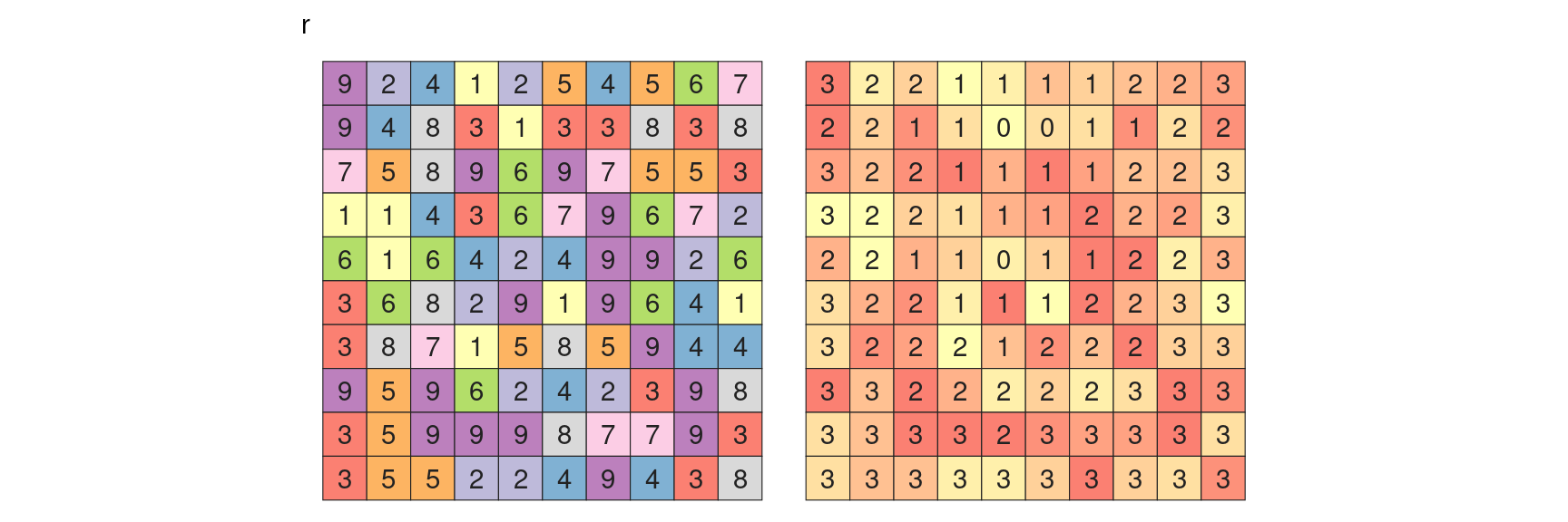
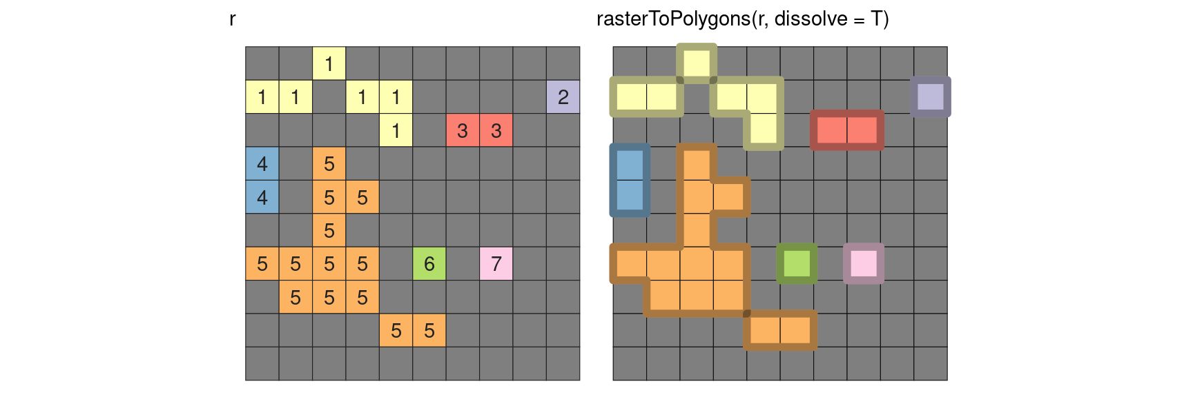
boundaries

“Detect boundaries (edges). boundaries are cells that have more than one class in the 4 or 8 cells surrounding it, or, if classes=FALSE, cells with values and cells with NA.”

extract

extract(r, pt)
#> [1] 8
extract(r, ln)
#> [[1]]
#>  [1] 6 7 6 4 2 6 8 8 9 5 3
extract(r, poly)
#> [[1]]
#>  [1] 6 9 3 6 7 9 2 4 9 9 1 9 5 8 5

rasterize

Note that polygon rasterization is by default looking at cell centroid overlap,

Statistical

Statistical operations summarize the raster information

density

density(r)

histogram

hist(r)

Spatial autocorrelation

Moran(r)
Geary(r)

Geometric

extent

extent(r)

crop

e = extent(0.23, 0.86, 0.22, 0.73)

intersect

g = extent(0.43, 1.1, -0.1, 0.53)

cellsFromExtent

cellsFromExtent(r, g)
#>  [1]  55  56  57  58  59  60  65  66  67  68  69  70  75  76  77  78  79  80  85
#> [20]  86  87  88  89  90  95  96  97  98  99 100

union

union(extent(r), g)

flip

flip(r_split, "y")

extend

mosaic

rasterToPoints

pts = rasterToPoints(r)

rasterToPolygons

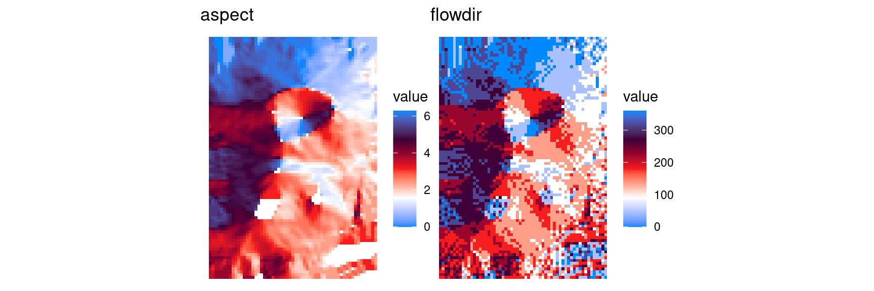
Terrain

terrain

r_terrain = terrain(v, opt = c("slope", "aspect", "tpi", "tri", "roughness", "flowdir"))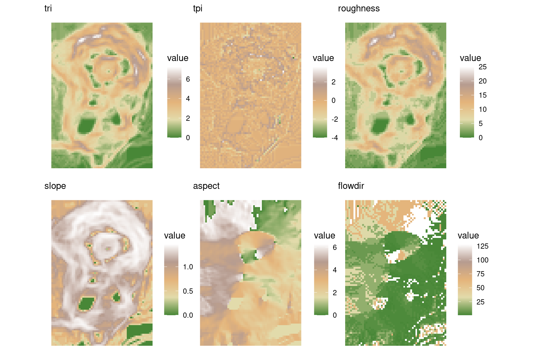

Angular data can sometimes be better expressed using a circular palette. In the following figure, blue is North orientation, while South is red. Both colors reach black at West and white at East. The preceeding figure had some sharp edges on North faces, when angle slightly changed from 360 to 0.

hillShade

r_hill = hillShade(r_terrain[["slope"]], r_terrain[["aspect"]])

interpolate

tps = Tps(survey[, c("x", "y")], survey$layer)
r_interpolate = interpolate(v, tps)