Working with hafvog data • ovog

Preamble

The primary purpose of {hafvog} is to extract, import and reformat the json files that are stored in the zip-file generated when exporting data from the hafvog proper software.

Installing

To install it do:

remotes::install_github("einarhjorleifsson/ovog")

library(tidyverse)
library(ovog)
library(tidyverse)

Importing

Importing is done via ‘hv_import’. One normally would do something like this (replace the name with whatever zip-name you have on your computer):

res <- hv_import(zipfiles = "A7-2024.zip")

For a demo we will download a zip file from hafro ftp-site:

tmpfile <- tempfile()
download.file("ftp://ftp.hafro.is/pub/data/A7-2024.zip", destfile = tmpfile)
res <- hv_import(tmpfile)
names(res)
#> [1] "stodvar"        "skraning"       "leidangrar"     "drasl_skraning"

The imported object is a list that contains the following tibbles: leidangrar, stodvar, skraning and drasl_skraning. Besides the table stodvar the other key measuements table is skraning. The latter table may not be familiar to those that work from the main Oracle database, but in essence it contains all biological measurements from simple count to prey content of predators.

We one can access any of the table in the list via:

res$skraning |> glimpse()
#> Rows: 1,733
#> Columns: 20
#> $ leidangur             <chr> "A7-2024", "A7-2024", "A7-2024", "A7-2024", "A7-…
#> $ synis_id              <int> 1, 1, 1, 1, 1, 1, 1, 1, 1, 1, 1, 1, 1, 1, 1, 1, …
#> $ maeliadgerd           <int> 3, 3, 3, 3, 3, 3, 3, 3, 3, 3, 3, 3, 3, 3, 3, 3, …
#> $ tegund                <int> 11, 209, 209, 209, 209, 209, 209, 209, 209, 209,…
#> $ lengd                 <dbl> 36.0, 6.6, 6.9, 4.8, 5.9, 4.5, 6.0, 5.4, 6.2, 4.…
#> $ fjoldi                <int> 1, 1, 1, 1, 1, 1, 1, 1, 1, 1, 1, 1, 1, 1, 1, 1, …
#> $ kyn                   <dbl> 2, NA, NA, NA, NA, NA, NA, NA, NA, NA, NA, NA, N…
#> $ kynthroski            <dbl> 33, NA, NA, NA, NA, NA, NA, NA, NA, NA, NA, NA, …
#> $ kvarnanr              <int> NA, NA, NA, NA, NA, NA, NA, NA, NA, NA, NA, NA, …
#> $ nr                    <int> 1, 1, 2, 3, 4, 5, 6, 7, 8, 9, 10, 11, 12, 13, 14…
#> $ oslaegt               <dbl> 494.00, 2.76, 3.66, 0.98, 1.92, 1.06, 2.30, 1.58…
#> $ slaegt                <dbl> NA, NA, NA, NA, NA, NA, NA, NA, NA, NA, NA, NA, …
#> $ magaastand            <dbl> 2, NA, NA, NA, NA, NA, NA, NA, NA, NA, NA, NA, N…
#> $ lifur                 <dbl> 2, NA, NA, NA, NA, NA, NA, NA, NA, NA, NA, NA, N…
#> $ kynfaeri              <dbl> NA, NA, NA, NA, NA, NA, NA, NA, NA, NA, NA, NA, …
#> $ tegund_as_faedutegund <int> 11, 209, 209, 209, 209, 209, 209, 209, 209, 209,…
#> $ radnr                 <int> 1, 2, 3, 4, 5, 6, 7, 8, 9, 10, 11, 12, 13, 14, 1…
#> $ ranfiskurteg          <int> NA, NA, NA, NA, NA, NA, NA, NA, NA, NA, NA, NA, …
#> $ heildarthyngd         <dbl> NA, NA, NA, NA, NA, NA, NA, NA, NA, NA, NA, NA, …
#> $ valkvorn              <lgl> FALSE, FALSE, FALSE, FALSE, FALSE, FALSE, FALSE,…

Some transformations

One can get the more familiar “kvarnir”, “lengdir” and “numer” (talning) format from the “skraning” table by passing the list object to the ‘hv_create_tables’-function:

res <- 
  res |> 
  hv_create_tables()
res |> names()
#> [1] "stodvar"  "skraning" "numer"    "lengdir"  "kvarnir"  "pp"

To access e.g. the “numer” table one does:

res$numer |> glimpse()
#> Rows: 940
#> Columns: 7
#> $ leidangur <chr> "A7-2024", "A7-2024", "A7-2024", "A7-2024", "A7-2024", "A7-2…
#> $ synis_id  <int> 1, 1, 1, 1, 1, 1, 1, 1, 1, 1, 1, 1, 1, 1, 1, 1, 1, 1, 1, 1, …
#> $ tegund    <int> 5, 11, 34, 44, 61, 71, 75, 100, 104, 106, 107, 111, 116, 120…
#> $ fj_maelt  <int> 0, 1, 0, 0, 0, 0, 0, 0, 0, 0, 0, 0, 0, 0, 0, 0, 0, 0, 0, 20,…
#> $ fj_talid  <int> 0, 0, 0, 0, 0, 0, 0, 0, 0, 0, 0, 0, 0, 0, 0, 0, 0, 0, 0, 25,…
#> $ fj_alls   <int> 0, 1, 0, 0, 0, 0, 0, 0, 0, 0, 0, 0, 0, 0, 0, 0, 0, 0, 0, 45,…
#> $ r         <dbl> 1.00, 1.00, 1.00, 1.00, 1.00, 1.00, 1.00, 1.00, 1.00, 1.00, …

One could e.g. plot the station location via:

res$stodvar |> 
  ggplot(aes(-kastad_v_lengd, kastad_n_breidd)) +
  geom_point() +
  coord_quickmap()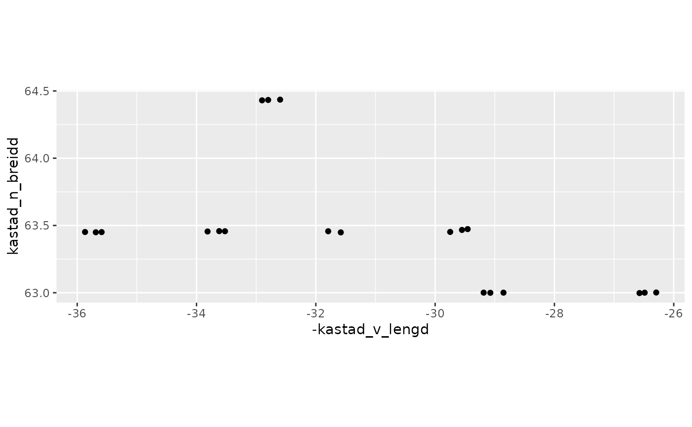

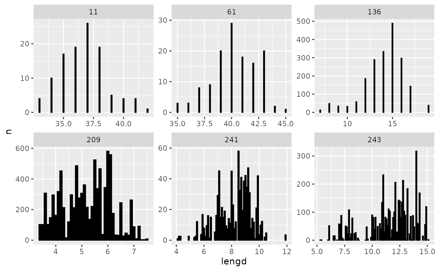
Or one could e.g. take a peek at the length distribution by the familiar:

res$lengdir |> 
  filter(tegund %in% c(209, 243, 136, 241, 164, 61, 11)) |> 
  group_by(tegund, lengd) |> 
  reframe(n = sum(n)) |> 
  ggplot(aes(lengd, n)) +
  geom_col(fill = "black", colour = "black") +
  facet_wrap(~ tegund, scales = "free")