demo
emulation.RmdReading data from dumped zip-files
One can read in the data currently being collected using the
hv_import_cruise that resides in the {ovog}-package:
cruises <- here::here(c("data-raw/TB2-2024.zip", "data-raw/TTH1-2024.zip"))
measurement <-
  ovog::hv_import(cruises) |>
  ovog::hv_create_tables()
The object returned is a list containing the following tables:
names(measurement)
#> [1] "stodvar"  "skraning" "numer"    "lengdir"  "kvarnir"  "pp"
Explorations - A sidestep
There should be nothing stopping you from doing analysis of the this data, e.g. one can easily get an overview of the reported station location via:
measurement$stodvar |>
  ggplot() +
  theme_bw() +
  geom_segment(aes(x = -kastad_v_lengd, y = kastad_n_breidd,
                   xend = -hift_v_lengd, yend = hift_n_breidd,
                   colour = factor(fishing_gear_no)),
               linewidth = 1) +
  coord_quickmap()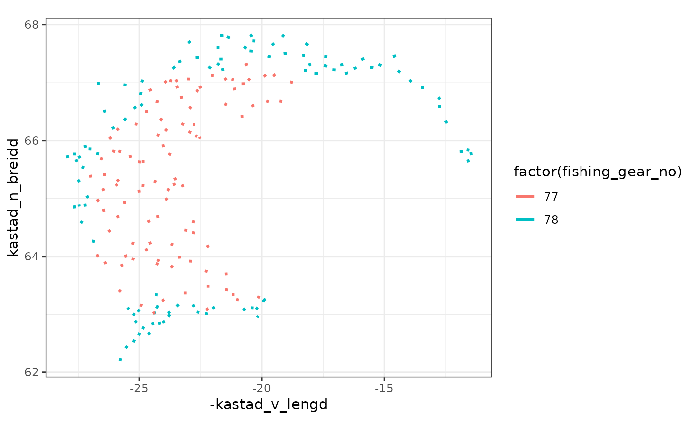
Or just the length distributions of some selected species via:
measurement$lengdir |>
  filter(tegund %in% 1:3) |>
  group_by(tegund, lengd) |>
  reframe(n = sum(n)) |>
  ggplot(aes(lengd, n)) +
  geom_col() +
  facet_wrap(~ tegund, scales = "free_y")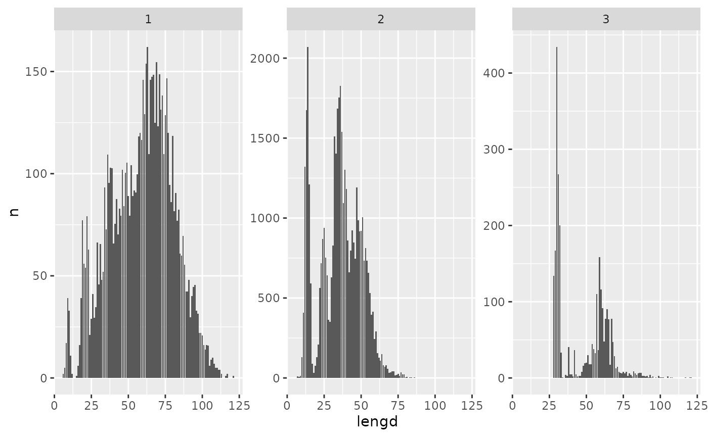
Merging and data transformation
Normally we would …
cruises <- here::here(c("data-raw/TB2-2024.zip", "data-raw/TTH1-2024.zip"))
stillingar <- here::here("data-raw/stillingar_SMH_rall_(haust).zip")
stodtoflur <- here::here("data-raw/stodtoflur.zip")
res <- sm_munge(cruises, stillingar, stodtoflur)
#> IMPORT
#> Import current measurements
#> The 'synaflokkur' of the zip files is: 35
#> Import setup ('stillingar')
#> Rename variables in sti_rallstodvar
#> Import setup ('stodtoflur')
#> Importing historical measurements (takes a while)
#> Combine current and historical data
#> MUNGE
#> Scale by counted
#> Standardize to towlength
#> Results by year and length
#> Results by station
#>
#> Trawl metrics and temperature
#> Time series
#> Last 20 tows
#> Tidy 'Stillingar'
#> 'Length-weight'
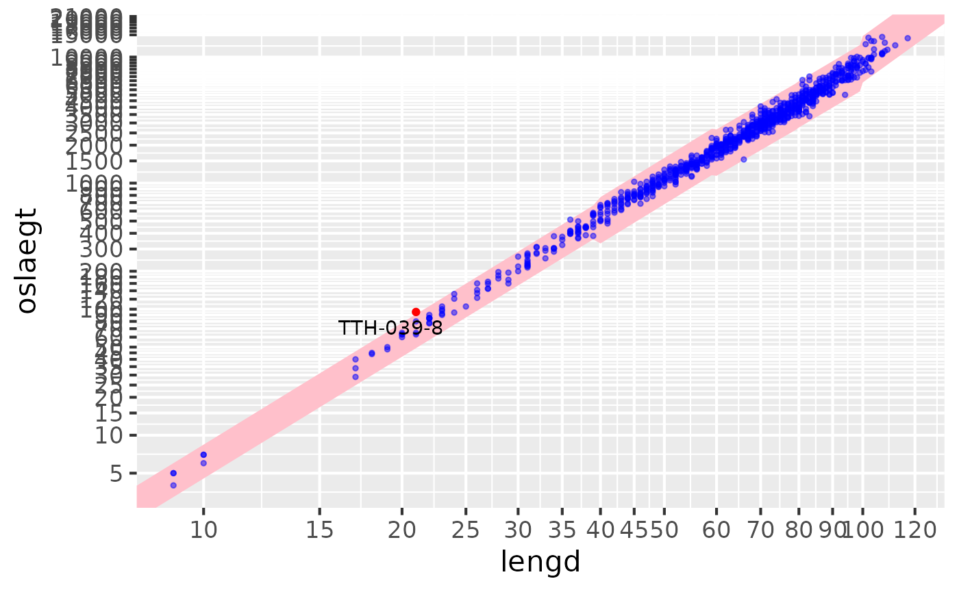
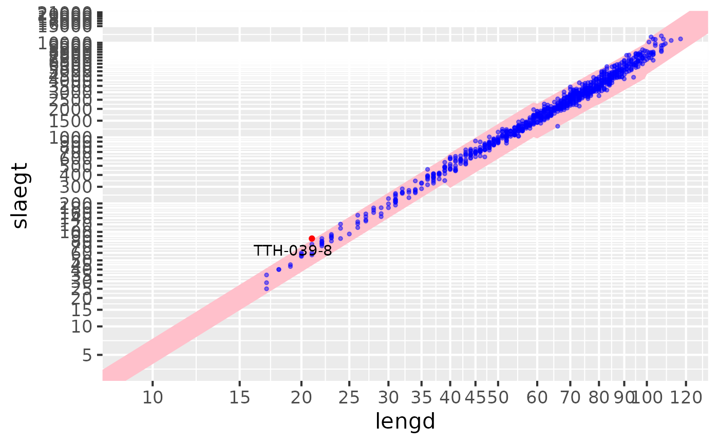
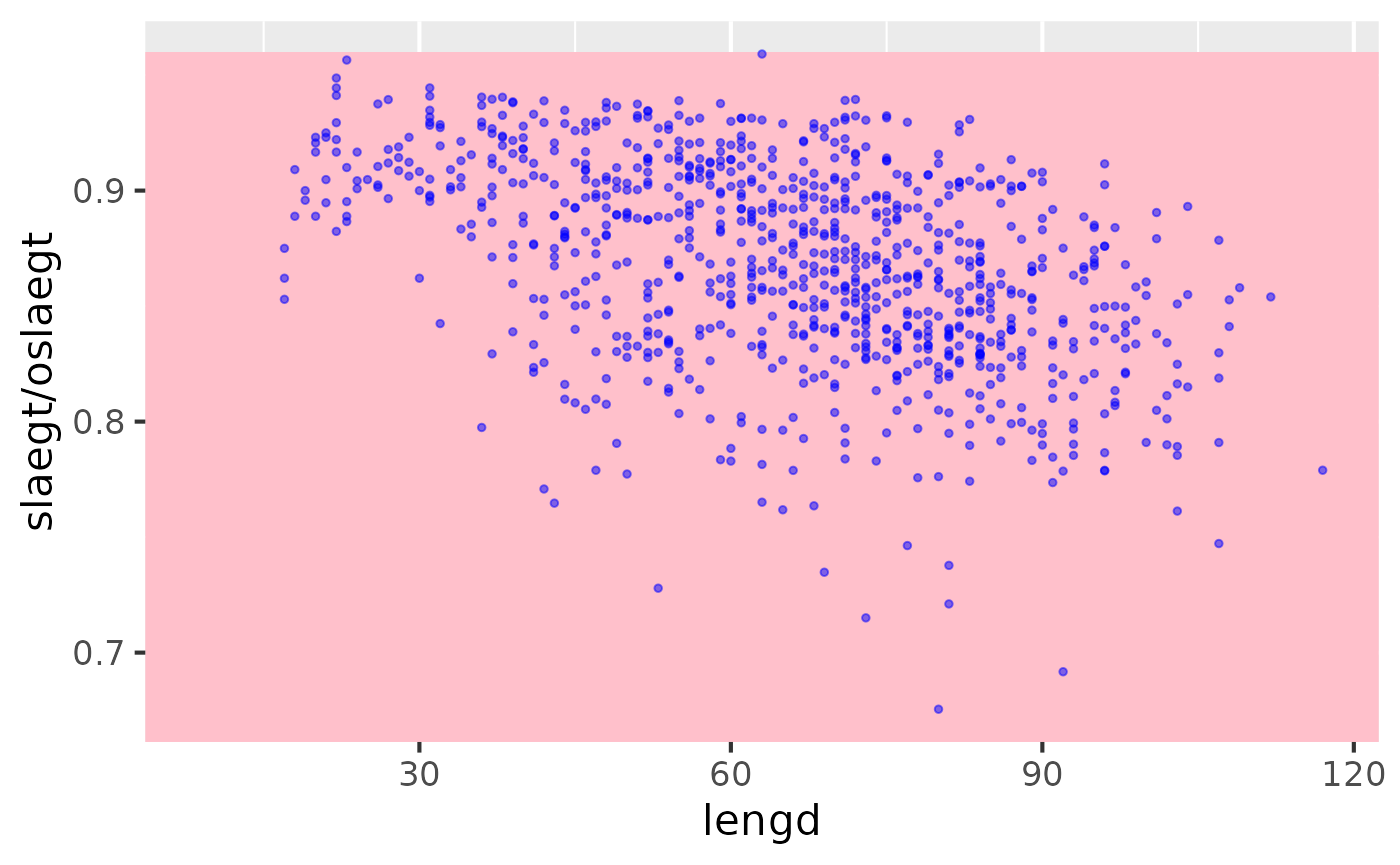
#> Checking measurments
#> Checking length vs weights
#> Checking gutted, gonads, liver vs ungutted ratio
#> REMINDER: Need to get data on magi
#> Formatting QC table
#> Togfar
#> Handbokartog
#> Valblod
#> Bootstrapping abundance
#>
#> Bootstrapping biomass
#>
#> HURRA! Exploration outside the smx-app
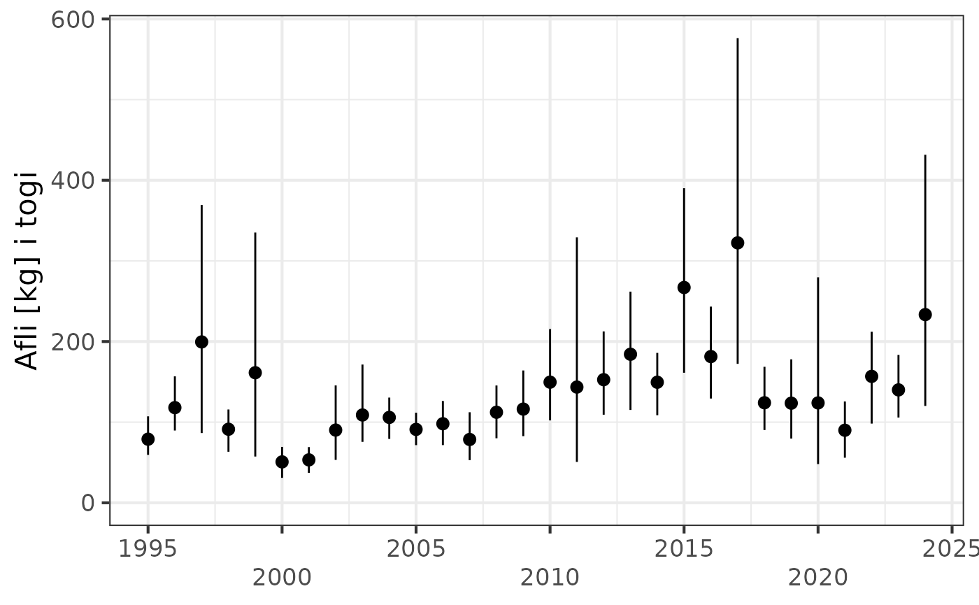
Sum of catch by lengths
res$by.length |>
  dplyr::filter(tegund == 1,
                ar >= 2010) |>
  dplyr::filter(var == "n") |>
  sm_plot_lengths()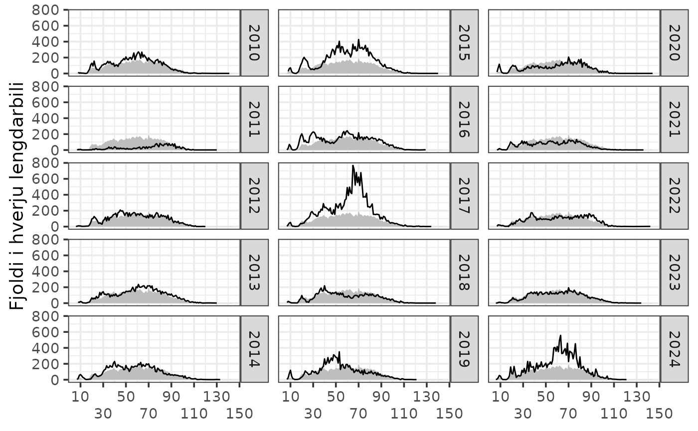
Catch by station
res$by.station |>
  dplyr::filter(tegund == 1,
                var == "b",
                ar %in% c(seq(2000, 2015, by = 5),
                          2017:2024)) |>
  sm_plot_bubble()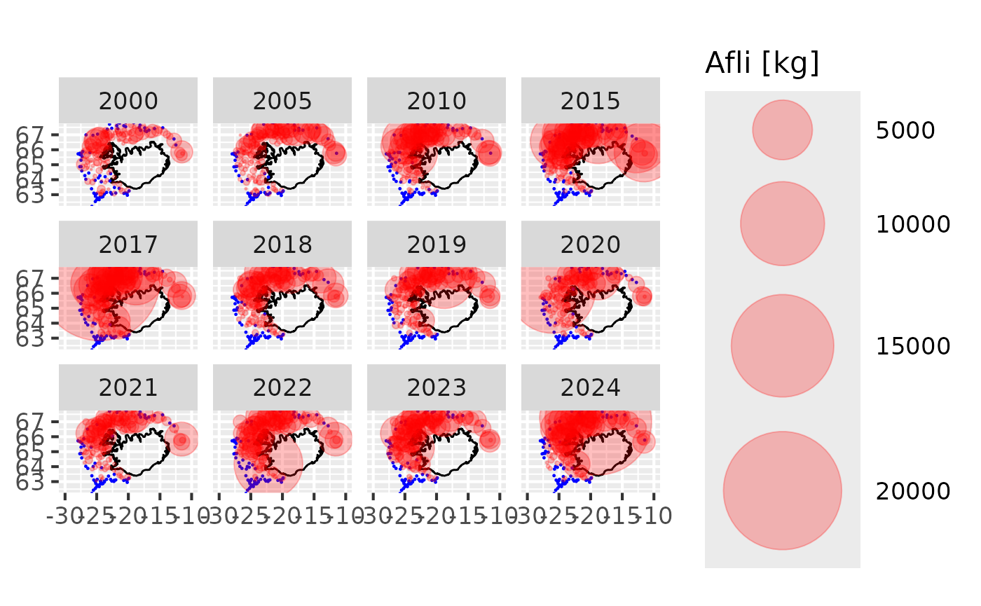
Catch by square
res$by.rect |>
  dplyr::filter(tegund == 1,
                var == "n") |>
  sm_plot_glyph()
#> Registered S3 method overwritten by 'GGally':
#>   method from
#>   +.gg   ggplot2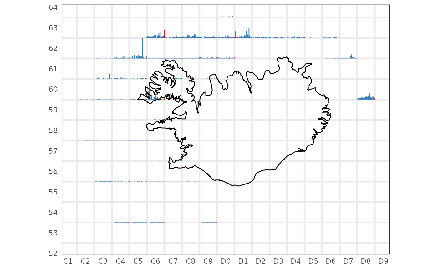
res$by.rect |>
  dplyr::filter(tegund == 2,
                var == "b") |>
  sm_plot_glyph()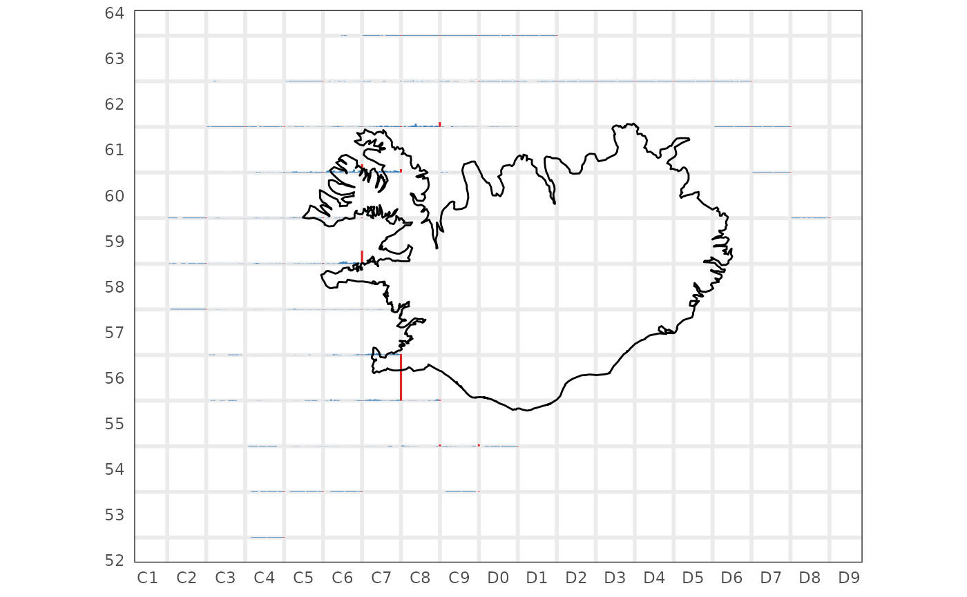
Probability of capture
tmp <-
  res$by.station |>
  dplyr::filter(ar == max(ar), tegund == 22, var == "n") |>
  dplyr::mutate(val = ifelse(val == 0, "absent", "present")) |>
  dplyr::select(lon, lat, val)
res$p_capture |>
  dplyr::filter(tegund == 22) |>
  sm_plot_probability() +
  ggplot2::geom_point(data = tmp,
                      ggplot2::aes(lon, lat, colour = val),
                      size = 0.5) +
  ggplot2::scale_colour_manual(values = c("present" = "cyan", "absent" = "white"),
                               guide = "none")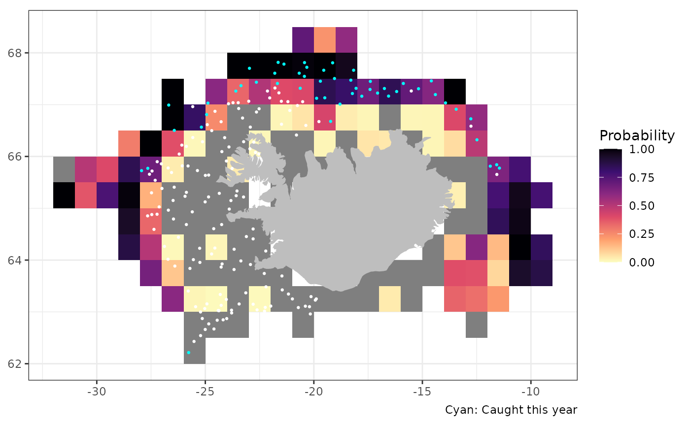
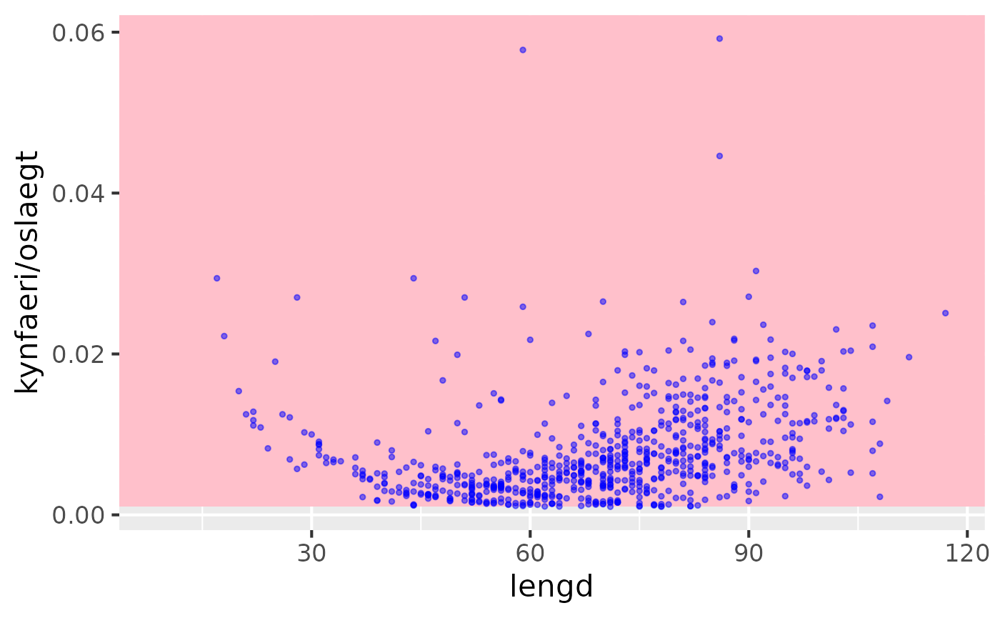
Lengths vs liver / ungutted
res |> sm_plot_liver()
#> Warning: Removed 3 rows containing missing values or values outside the scale range
#> (`geom_point()`).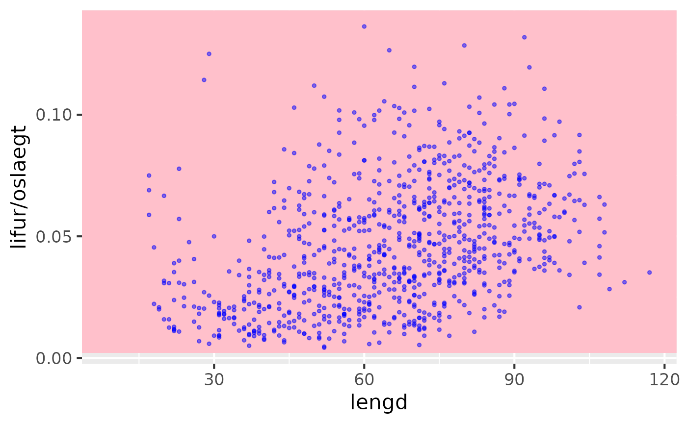
Prey table
res$pp |>
  dplyr::filter(astand %in% 1) |>
  osmx::sm_table_prey()
Prey histogram
### Þyngdardreifing á bráð - Topp 20 bráðir

# applly some filter
pp <-
  res$pp |>
  dplyr::filter(astand == 1,
                # brað verdur ad vera skilgreind
                !is.na(prey),
                # verður að hafa mælingu thyngd
                !is.na(heildarthyngd),
                # verður að hafa mælingu talid
                !is.na(n)) |>
  dplyr::mutate(m.thyngd = round(heildarthyngd / n, 2))

# not really mean based on individual prey measurements
pp.mean <-
  pp |>
  dplyr::group_by(prey) |>
  dplyr::summarise(fjoldi = sum(n),
                   mean = sum(heildarthyngd) / sum(n)) |>
  dplyr::ungroup() |>
  dplyr::arrange(-fjoldi)

# top 20 (bráð) tegundir "mældar"
top20 <-
  pp.mean |>
  dplyr::slice(1:20)
top20.brad <-
  top20 |>
  dplyr::pull(prey)

pp |>
  dplyr::filter(prey %in% top20.brad) |>
  ggplot2::ggplot() +
  ggplot2::geom_histogram(ggplot2::aes(m.thyngd)) +
  ggplot2::geom_vline(data = top20,
                      ggplot2::aes(xintercept = mean), colour = "red") +
  ggplot2::facet_wrap(~ prey, scale = "free") +
  ggplot2::labs(x = "Meðalþyngd", y = "Fjöldi")
#> `stat_bin()` using `bins = 30`. Pick better value with `binwidth`.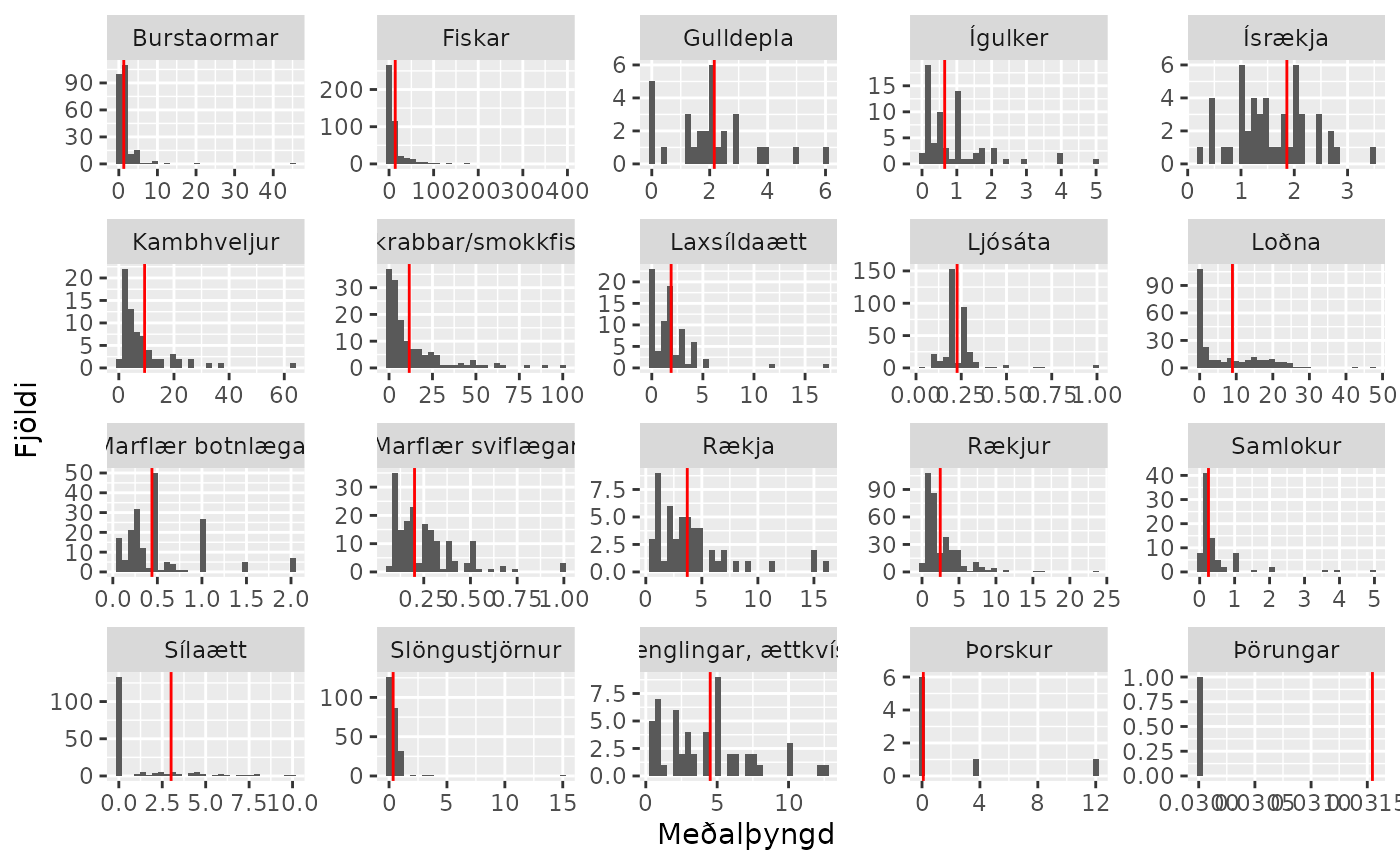
Pred-prey figures
tmp |>
  ggplot2::ggplot() +
  ggplot2::geom_histogram(ggplot2::aes(magafylli)) +
  ggplot2::facet_wrap(~ fiskur, scales = "free")
#> `stat_bin()` using `bins = 30`. Pick better value with `binwidth`.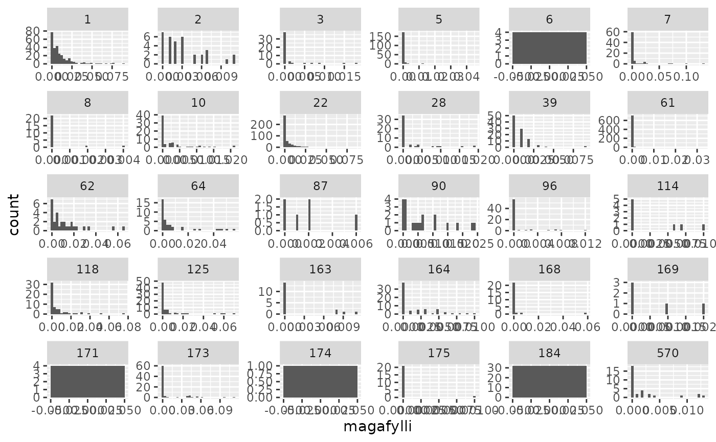
res$kv.this.year |>
  dplyr::filter(leidangur %in% "TB2-2024") |>
sm_table_kvarnir()Gear metrics - last 20 stations
res$timetrend.20 |>
  filter(leidangur %in% "TB2-2024",
         var %in% c("larett_opnun", "lodrett_opnun", "vir_uti")) |>
  sm_plot_last20()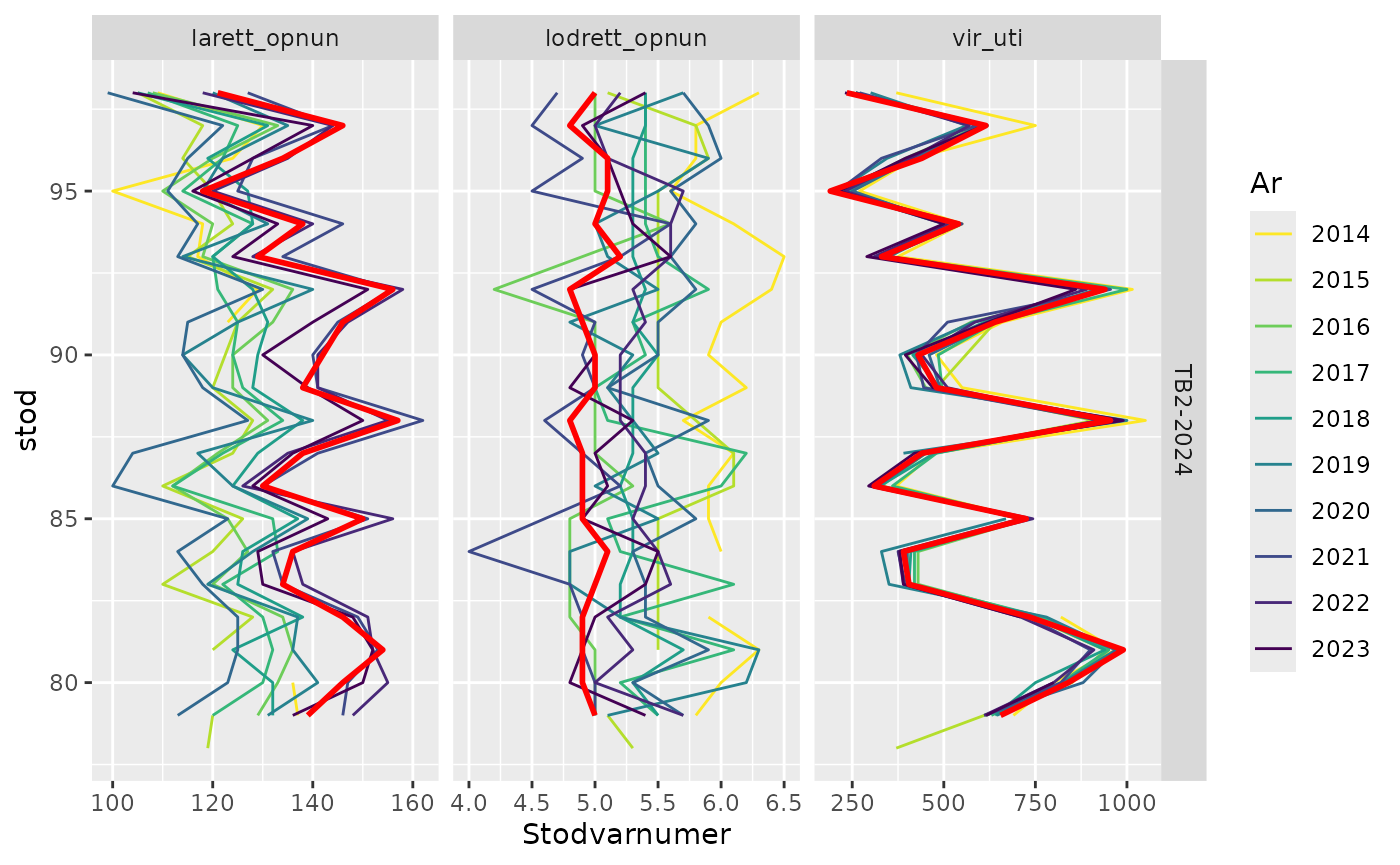
Temperatures - last 20 stations
res$timetrend.20 |>
  filter(leidangur %in% "TB2-2024",
         var %in% c("botnhiti", "yfirbordshiti")) |>
  sm_plot_last20()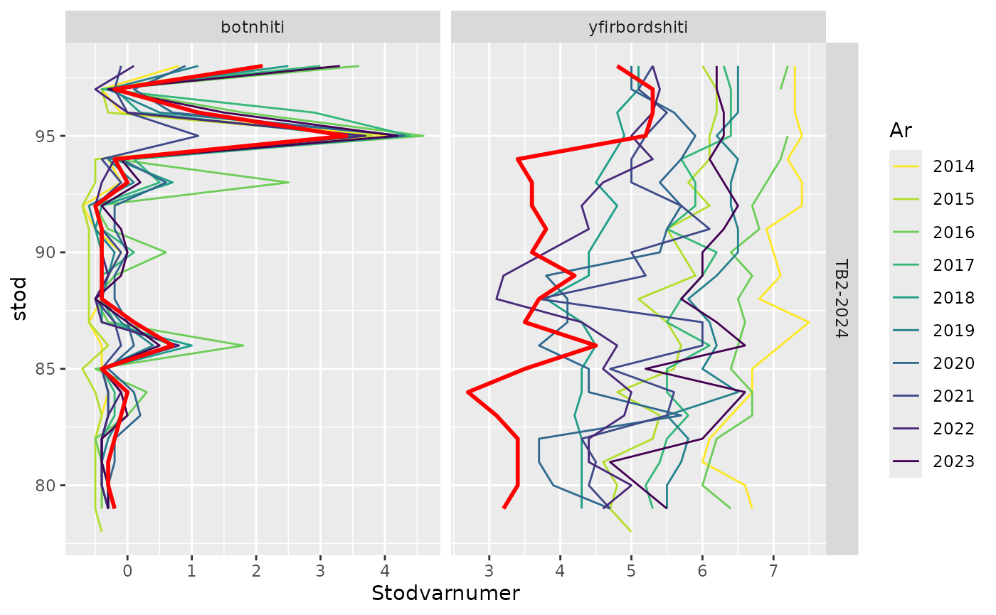
Gear metrics - time trends
res$timetrend |>
  filter(leidangur %in% "TB2-2024",
         var %in% c("larett_opnun", "lodrett_opnun", "vir_uti")) |>
  sm_plot_violin()
#> Warning: Removed 943 rows containing non-finite outside the scale range
#> (`stat_ydensity()`).
#> Warning: Removed 943 rows containing missing values or values outside the scale range
#> (`geom_point()`).
#> Warning: Removed 5 rows containing missing values or values outside the scale range
#> (`geom_line()`).
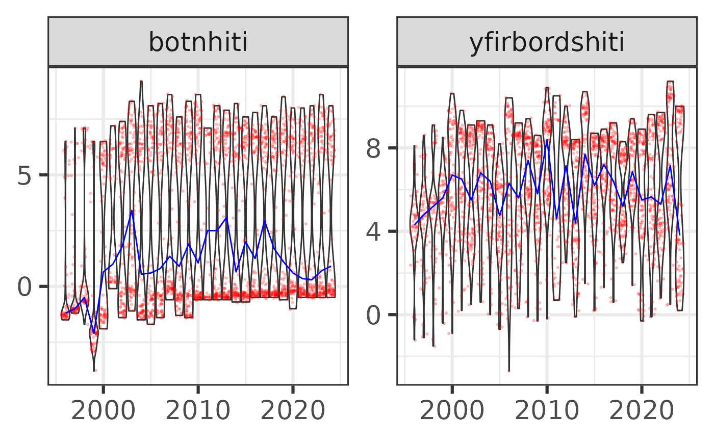
Temperature - time trends
res$timetrend |>
  filter(leidangur %in% "TB2-2024",
         var %in% c("botnhiti", "yfirbordshiti")) |>
  sm_plot_violin()
#> Warning: Removed 115 rows containing non-finite outside the scale range
#> (`stat_ydensity()`).
#> Warning: Removed 115 rows containing missing values or values outside the scale range
#> (`geom_point()`).