EDA • fmr

library(fmr)
library(tidyverse)
library(here)

Preamble

This document is just to explore the FM data model, done to prevent any misunderstanding when setting up the downstream code. In addition it deals with some issues and questions that arise related to the data-entry of catch-sample data.

The FM API on is made up from three tables (The Data Structured Explained).

Survey table - distinguished by survey_id
Survey detail table - distinguished by survey_item_id
Survey item table - distinguished by survey_item_dtl_id

The conceptual design (if one is considering catch-sampling on landing sites) is depicted as:

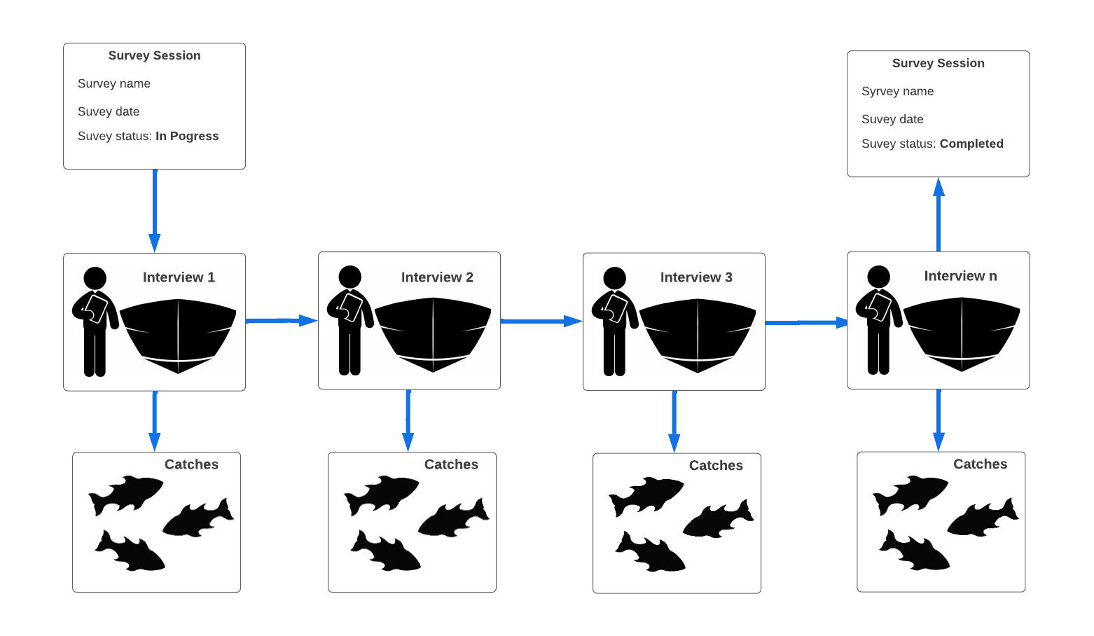
Source: Fisheries Technologies.

The FM 3 table framework is not specific for sampling from landings, but lets here think about these three tables in that context.

Sampling site table (survey table): For catch-sampling from landings data one could imagine that each record represents information about the sampling from a particular sampling site on a particular sampling date (this though not the necessary case as discussed below).
Trip table (surveyitem table): In case of catch sampling from landings this table should contain all information related to a single fishing trip except details of catch.
Catch table (surveyitem detail table): In case of catch sampling from landings this table will contain the detailed information about catch by species.

The connection

…

key <- "your_FM_API_key"

The three survey tables

Let’s start by loading in tables needed, if only because we need information from the downstream tables to make sense of the upstream tables:

survey <- fm_survey(key)
trip <- fm_trip(key)
catch <- fm_catch(key)

The landing site-date table (Survey table)

survey |> glimpse()
#> Rows: 3,033
#> Columns: 10
#> $ site        <chr> "Basseterre West", "Sandy Point", "Basseterre East", "Bass…
#> $ island      <chr> "Saint Kitts", "Saint Kitts", "Saint Kitts", "Saint Kitts"…
#> $ status      <chr> "Completed", "Completed", "Completed", "Completed", "Compl…
#> $ date        <date> 2023-02-15, 2023-01-11, 2023-01-08, 2023-01-08, 2023-01-0…
#> $ T1          <dttm> 2023-02-15 05:50:00, 2023-01-11 14:00:00, 2023-01-08 16:0…
#> $ T2          <dttm> 2024-02-15 16:00:00, 2023-01-11 23:00:00, 2023-01-08 20:0…
#> $ total_boats <dbl> 1, 1, 4, 4, 4, 12, 4, 4, 1, 1, 1, 6, 1, 6, 10, 10, 10, 6, …
#> $ type        <chr> "Landing", "Landing", "Landing", "Landing", "Landing", "La…
#> $ collector   <chr> "Enver Pemberton", "Doret Williams", NA, NA, NA, "Judika E…
#> $ survey_id   <dbl> 1475, 1487, 1493, 1494, 1495, 1496, 1498, 1499, 1503, 1513…

Each survey is identified by a unique value stored as survey_id (survey_id). Intuitively one expects that each survey id constitutes a unique number for each landing site (site) by each sampling day (date). This is however not necessarily the case, as demonstrated below.

What does a single survey_id (survey_id) represent?

Let’s take a look at one month of data from one site:

d <- 
  survey |> 
  # look at one month
  filter(year(date) == 2024, month(date) == 1,
         site == "Basseterre East") |>
  arrange(date) |> 
  group_by(site, date) |> 
  summarise(n = n_distinct(survey_id),
            .groups = "drop")
d |> 
  knitr::kable(caption = "Number of surveys per date")

Number of surveys per date
site	date	n
Basseterre East	2024-01-04	3
Basseterre East	2024-01-05	2
Basseterre East	2024-01-06	2
Basseterre East	2024-01-07	2
Basseterre East	2024-01-08	2
Basseterre East	2024-01-09	1
Basseterre East	2024-01-10	2
Basseterre East	2024-01-11	2
Basseterre East	2024-01-12	2
Basseterre East	2024-01-14	1
Basseterre East	2024-01-16	3
Basseterre East	2024-01-17	3
Basseterre East	2024-01-19	1
Basseterre East	2024-01-22	1
Basseterre East	2024-01-23	1
Basseterre East	2024-01-24	1
Basseterre East	2024-01-26	1
Basseterre East	2024-01-29	1
Basseterre East	2024-01-30	2
Basseterre East	2024-01-31	5

Visually we have:

d |> 
  mutate(survey = TRUE) |> 
  fm_grid_calendar() |> 
  mutate(weekend = ifelse(.wday %in% c("Sa", "Su"),
                          TRUE,
                          FALSE),
         survey = replace_na(survey, FALSE)) |> 
  ggplot(aes(.wday, .week)) +
  theme_bw() +
  geom_tile(aes(fill = survey),
            colour = "black") +
  facet_wrap(~ site) +
  geom_text(aes(label = .day, colour = weekend)) +
  geom_text(aes(label = n), nudge_x = 0.2, nudge_y = -0.2,
            size = 3, colour = "blue") +
  scale_fill_manual(values=c("grey80", "pink")) +
  scale_colour_manual(values = c("black", "red")) +
  scale_y_reverse(NULL, NULL) +
  labs(x = NULL,
       title = "March 2024",
       caption = "Colour: pink - reported sampling day, blue - number of surveys") +
  coord_equal() +
  theme(legend.position = "none",
        legend.title=element_blank(), 
        panel.grid=element_blank(), 
        panel.border=element_blank(), 
        axis.ticks=element_blank(), 
        strip.background=element_blank(), 
        #legend.position="top", 
        legend.justification="right", 
        legend.direction="horizontal", 
        legend.key.size=unit(0.3, "cm"), 
        legend.spacing.x=unit(0.2, "cm"))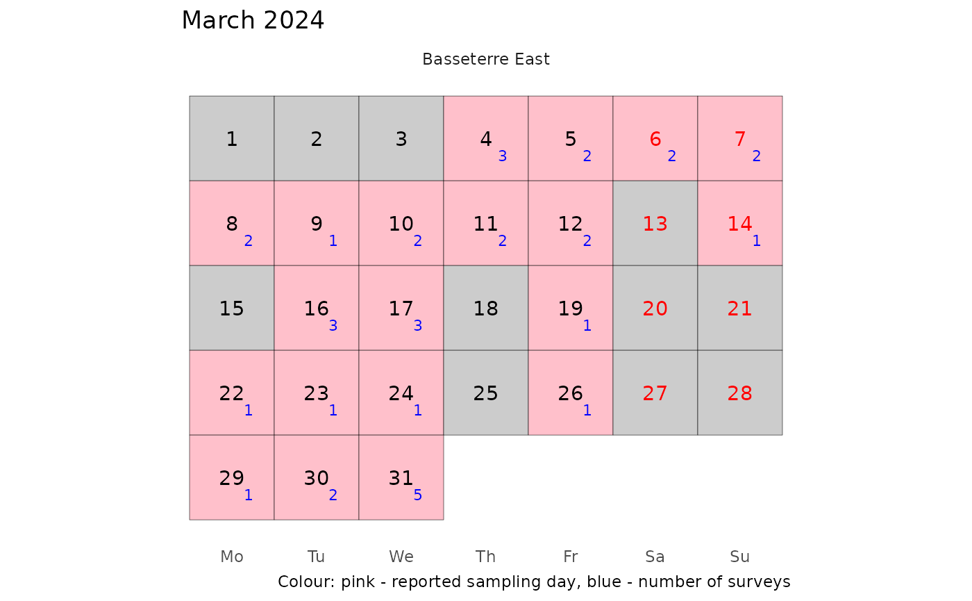

This is some dummy

Here the pink shade marks days that surveys were conducted and the blue colour represents the number of unique reported surveys. There are two points to observe here:

Having a survey date on a weekend is unexpected because observers do not work on those days.
The number of surveys per day are in many cases more than 1

Let’s look first at the weeend data:

# need to get the data again, now all variables
survey <- fm_survey(key, trim = FALSE)
d <- 
  survey |> 
  # look at one month
  filter(year(date) == 2024, month(date) == 1,
         site == "Basseterre East") |> 
  mutate(wday = wday(date, label = TRUE, locale = "en_GB.utf8")) |> 
  filter(wday %in% c("Sat", "Sun")) |> 
  count(survey_id, date, .cn, .ct, .un, .ut) |> 
  arrange(date, .ct)
d
#> # A tibble: 5 × 7
#>   survey_id date       .cn   .ct                 .un   .ut                     n
#>       <dbl> <date>     <chr> <dttm>              <chr> <dttm>              <int>
#> 1      5523 2024-01-06 Alli… 2024-01-11 15:34:50 Kade… 2024-01-12 19:05:31     1
#> 2      5803 2024-01-06 Alli… 2024-02-02 17:27:29 Kade… 2024-02-02 18:46:44     1
#> 3      5524 2024-01-07 Alli… 2024-01-11 15:39:21 Kade… 2024-01-12 19:04:37     1
#> 4      5592 2024-01-07 Asho… 2024-01-17 23:08:20 Kade… 2024-01-18 14:29:45     1
#> 5      5840 2024-01-14 Asho… 2024-02-06 12:25:28 Kade… 2024-02-06 18:18:58     1

Here we see that we have:

3 survey weekdays
In each case the creation date (.ct) is not the same as the survey date
On one date (2024-01-07) we have two persons creating a survey on two separated dates

The most likely explanation is that these surveys are actually informations obtained from the fishermen and that the survey date was set the same as the fishing day. To check this we need to dig into downstream tables:

survey |> 
  filter(survey_id %in% d$survey_id) |> 
  select(survey_id, date, .ct, .cn) |> 
  left_join(trip |> select(vessel, regno, t1, t2, survey_id, .s2)) |> 
  left_join(catch |> select(.s2, type = measurement_type) |> distinct()) |>  
  arrange(date, .cn) |> 
  knitr::kable()
#> Error in `select()`:
#> ! Can't select columns that don't exist.
#> ✖ Column `t1` doesn't exist.

Here one observes the measurement type is in two cases FE () but unexpectedly WT () in three cases. The table above gives rise to three QC points:

QC01: If fishing on weekend should one not expect that the measurement_type is FE
QC02: Should one expect that one can only have one record (trip) per vessel per fishing day
      Related, one can not have overlapping trip time (t1 to t2) for the same vessel
QC03: Should one exepect that fishing period is more than ~1 day, i.e. are there multi-day-trips
      Would this depend on gear type

Ad hoc question:

s1 |> 
  select(survey_id, date, .cn, .ct) |> 
  filter(year(date) == 2024) |> 
  inner_join(s2 |> select(vid, survey_id, .s2, t1, t2)) |> 
  inner_join(s3 |> select(.s2, type = measurement_type) |> distinct()) |> 
  select(vid, date, type, t1, t2, everything()) |> 
  arrange(vid, date, type) |> 
  group_by(vid, date, type) |> 
  mutate(n = n(), .after = type) |> 
  ungroup() |> 
  filter(n > 1) |> 
  knitr::kable()
#> Error in eval(expr, envir, enclos): object 's1' not found

One could implement a unique id within the R-function, named e.g. .sid. We can test that via:

s1 <- 
  s1 |> 
  # just so we can get the original order back
  mutate(.rowid = 1:n()) |> 
  arrange(site, date, T1) |> 
  mutate(.sid = dplyr::consecutive_id(site, date)) |> 
  arrange(.rowid) |> 
  select(-.rowid)
#> Error in eval(expr, envir, enclos): object 's1' not found
s1 |> 
  summarise(n_sid = n_distinct(.sid),
            n_surveyid = n_distinct(survey_id),
            .groups = "drop")
#> Error in eval(expr, envir, enclos): object 's1' not found

One would use this table e.g. to get an overview of the reported sampled dates:

fm_survey(key, trim = FALSE) %>% 
  filter(year(date) == 2024,
         month(date) == 1) |> 
  select(site, date) |> 
  distinct() |> 
  mutate(survey = TRUE) |> 
  fm_grid_calendar() |> 
  mutate(weekend = ifelse(.wday %in% c("Sa", "Su"),
                          TRUE,
                          FALSE)) %>% 
  #filter(site == "Charlestown") |> 
  ggplot(aes(.wday, .week)) +
  theme_bw() +
  geom_tile(aes(fill = survey)) +
  facet_wrap(~ site) +
  geom_text(aes(label = .day, colour = weekend)) +
  scale_fill_manual(values=c("grey80", "pink")) +
  scale_colour_manual(values = c("black", "red")) +
  scale_y_reverse(NULL, NULL) +
  labs(x = NULL,
       title = "January 2024",
       caption = "colour: reported sampling day") +
  coord_equal() +
  theme(legend.position = "none",
        legend.title=element_blank(), 
        panel.grid=element_blank(), 
        panel.border=element_blank(), 
        axis.ticks=element_blank(), 
        strip.background=element_blank(), 
        #legend.position="top", 
        legend.justification="right", 
        legend.direction="horizontal", 
        legend.key.size=unit(0.3, "cm"), 
        legend.spacing.x=unit(0.2, "cm"))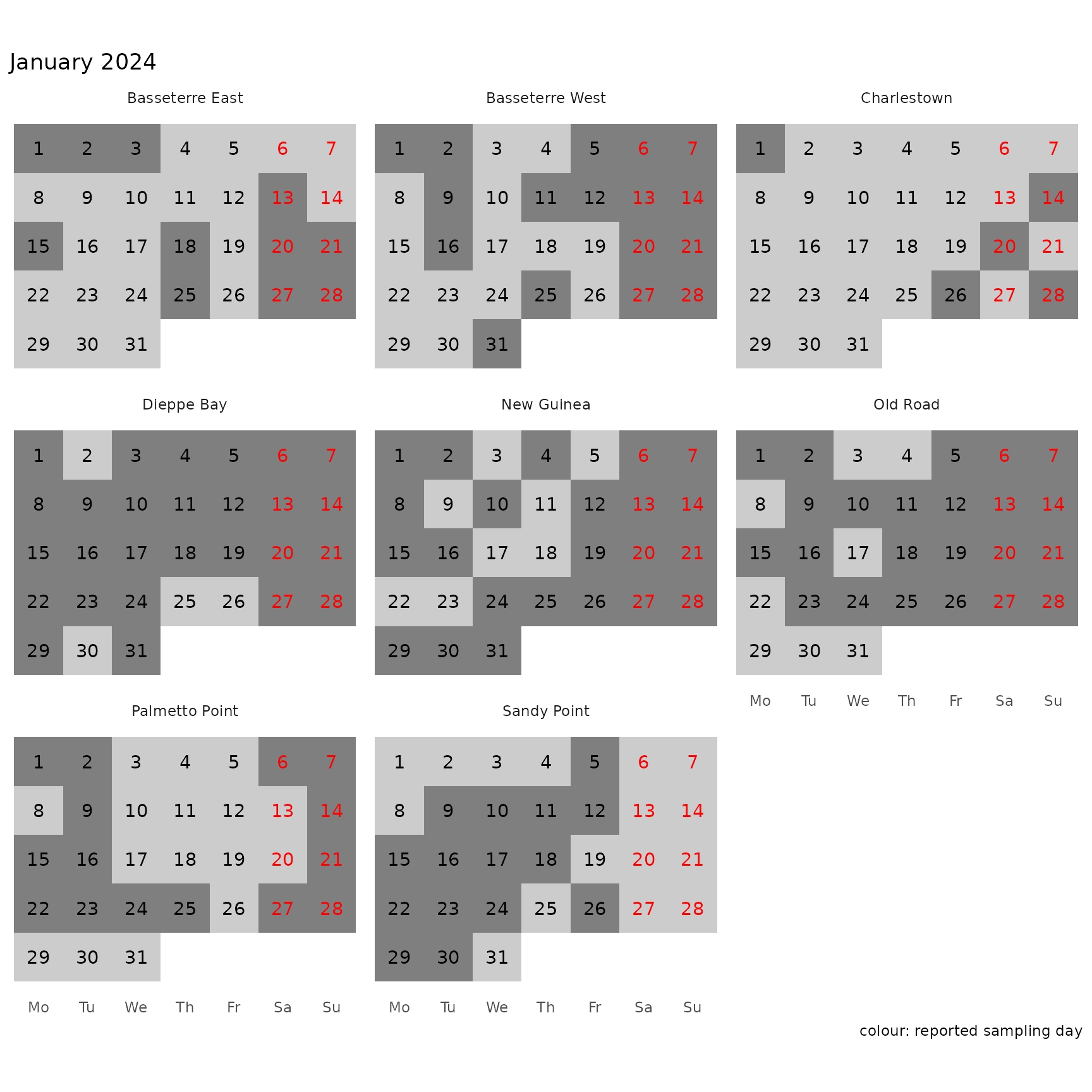

This is some dummy

Some issues

Do not expect that one can create a survey without a survey date:

s1 |> 
  filter(is.na(date)) |> 
  select(survey_id, site, date, status, T1, T2, n_boats = total_boats, comment,
         collector,
         .cn:.ut) |> 
  arrange(survey_id) |> 
  glimpse()
#> Error in eval(expr, envir, enclos): object 's1' not found

The surveyitem table

This is effectively the trip table.

QC: Expect only one trip per vessel per day

s2 |> 
  mutate(d1 = as_date(t1),
         d2 = as_date(t2)) |> 
  count(vid, d1) |> 
  count(n) |> 
  rename('Trips per day' = n, 
         'Number of records' = nn) |> 
  knitr::kable(caption = "Number of trips by vessels per day")
#> Error in eval(expr, envir, enclos): object 's2' not found

s2 |> 
  mutate(d1 = as_date(t1))
#> Error in eval(expr, envir, enclos): object 's2' not found

The surveyitemdtl table

s3 <- fmr::fm_surveyitemdtl(key)
#> Error: 'fm_surveyitemdtl' is not an exported object from 'namespace:fmr'
s3 |> glimpse()
#> Error in eval(expr, envir, enclos): object 's3' not found

The catch table (Survey item table)

pending further coding …

The wide tables

Combining these three data tables into a single wide-table is very common delivery approach when the downstream analysis is based on some kind of a spreadsheet software. The problem here though is that each measurements in the trip table gets repeated by the number of species recorded in the catch table and then the records associated with the sampling site get repeated by the number of trips. E.g. if on one sampling site within one day one samples 10 trips and for each of those 10 trips we measure 5 species we have 50 (10 trips x 5 species) repeated records of the variables associated with the sampling site table.

Wide-tables where one has repeated records of the same measure create a bit of a problem in statistical analysis, in particular when there are a lot of variables (columns) in such a wide-table. In order that any code generated is delivering what is intended the person using the wide-table has to have a full knowledge of the data-model in the first place. Which defies hence the logic of providing a wide table.

Of course on can access the wide tables provided by FM via {fmr} as shown below. Although wide tables are often used when using spreadsheet software, it is not recommended to use them for downstream analysis in R:

landing F

fm_landingF(key) |> glimpse()
#> Rows: 19,474
#> Columns: 37
#> $ id                    <int> 1, 2, 3, 4, 5, 6, 7, 8, 9, 10, 11, 12, 13, 14, 1…
#> $ survey_id             <int> 1478, 1484, 1484, 1484, 1489, 1492, 1492, 1492, …
#> $ survey_item_id        <int> 1517, 1523, 1523, 1523, 1529, 1532, 1532, 1532, …
#> $ survey_item_dtl_id    <int> 1691, 1703, 1706, 1707, 1718, 1724, 1725, 1727, …
#> $ survey_status_id      <int> 1807, 1807, 1807, 1807, 1807, 1807, 1807, 1807, …
#> $ survey_item_status_id <int> 1867, 1867, 1867, 1867, 1867, 1867, 1867, 1867, …
#> $ survey_item_type_id   <int> 1871, 1871, 1871, 1871, 1871, 1871, 1871, 1871, …
#> $ landing_date          <chr> "2023-01-05T10:00:00.000+00:00", "2023-01-09T10:…
#> $ landing_site_id       <int> 10081, 10081, 10081, 10081, 10081, 10080, 10080,…
#> $ vessel_id             <int> 2029, 2029, 2029, 2029, 1893, 1994, 1994, 1994, …
#> $ species_id            <int> 2254, 2174, 2291, 2407, 2458, 2303, 2126, 2237, …
#> $ weight                <dbl> 5, 12, 25, 40, 100, 12, 2, 5, 8, 3, 4, 150, 24, …
#> $ price                 <dbl> 12, 12, 12, 20, 10, 14, 12, 12, 12, 12, 12, 10, …
#> $ fuel_used             <dbl> NA, 500, 500, 500, 500, NA, NA, NA, NA, NA, NA, …
#> $ total                 <dbl> 60, 144, 300, 800, 1000, 168, 24, 60, 96, 36, 48…
#> $ gear_id               <int> 1081, 1081, 1081, 1081, 1080, 1081, 1081, 1081, …
#> $ fishing_zone_id       <int> 1085, 1085, 1085, 1085, 1085, 1085, 1085, 1085, …
#> $ condition_id          <int> 1877, 1877, 1877, 1877, 1877, 1877, 1877, 1877, …
#> $ infraction_type_id    <lgl> NA, NA, NA, NA, NA, NA, NA, NA, NA, NA, NA, NA, …
#> $ infraction_desc       <lgl> NA, NA, NA, NA, NA, NA, NA, NA, NA, NA, NA, NA, …
#> $ measurement_type_id   <lgl> NA, NA, NA, NA, NA, NA, NA, NA, NA, NA, NA, NA, …
#> $ disposition_id        <lgl> NA, NA, NA, NA, NA, NA, NA, NA, NA, NA, NA, NA, …
#> $ is_by_catch           <int> 1, 1, 1, 1, 1, 1, 1, 1, 1, 1, 1, 1, 1, 1, 1, 1, …
#> $ is_targetted          <int> 0, 0, 0, 0, 0, 0, 0, 0, 0, 0, 0, 0, 0, 0, 0, 0, …
#> $ storage_id            <lgl> NA, NA, NA, NA, NA, NA, NA, NA, NA, NA, NA, NA, …
#> $ dep_status_id         <int> 1861, 1861, 1861, 1861, 1861, 1861, 1861, 1861, …
#> $ dep_location_id       <int> 10081, 10081, 10081, 10081, 10081, 10080, 10080,…
#> $ dep_time              <chr> "2023-01-05T04:00:00.000+00:00", "2023-01-09T04:…
#> $ arr_location_id       <int> 10081, 10081, 10081, 10081, 10081, 10080, 10080,…
#> $ arr_status_id         <int> 1856, 1856, 1856, 1856, 1856, 1856, 1856, 1856, …
#> $ arr_time              <chr> "2023-01-05T16:00:00.000+00:00", "2023-01-09T16:…
#> $ secondary_gear_id     <lgl> NA, NA, NA, NA, NA, NA, NA, NA, NA, NA, NA, NA, …
#> $ secondary_vessel_id   <int> NA, NA, NA, NA, NA, NA, NA, NA, NA, NA, NA, NA, …
#> $ tenant_id             <int> 103, 103, 103, 103, 103, 103, 103, 103, 103, 103…
#> $ is_active             <int> 0, 0, 0, 0, 0, 0, 0, 0, 0, 0, 0, 0, 0, 0, 0, 0, …
#> $ created_by            <chr> "TracyG", "TracyG", "TracyG", "TracyG", "TracyG"…
#> $ created_date          <chr> "2023-02-15T16:26:01.467+00:00", "2023-02-16T01:…

landingV

fm_landingV(key) |> glimpse()
#> Rows: 19,474
#> Columns: 27
#> $ id                    <int> 1, 2, 3, 4, 5, 6, 7, 8, 9, 10, 11, 12, 13, 14, 1…
#> $ survey_id             <int> 7992, 7992, 7992, 7992, 7992, 7992, 7992, 7992, …
#> $ landing_date          <dttm> 2024-07-26 08:00:00, 2024-07-26 08:00:00, 2024-…
#> $ landing_date_time_str <dttm> 2024-07-26 08:07:00, 2024-07-26 08:07:00, 2024-…
#> $ landing_site_id       <int> 10080, 10080, 10080, 10080, 10080, 10080, 10080,…
#> $ landing_site          <chr> "Basseterre East", "Basseterre East", "Basseterr…
#> $ vessel_id             <int> 2260, 2260, 1881, 2260, 2260, 2263, 1881, 2260, …
#> $ vessel                <chr> "Nicholas", "Nicholas", "Lion Fish", "Nicholas",…
#> $ vessel_regno          <chr> "629BE", "629BE", "V4-542-BE", "629BE", "629BE",…
#> $ vessel_class_id       <int> 1041, 1041, 1029, 1041, 1041, 1041, 1029, 1041, …
#> $ vessel_class          <chr> "Vessels supporting fishing related activities",…
#> $ fishing_zone_id       <int> 1052, 1052, 1084, 1052, 1052, 1063, 1084, 1052, …
#> $ fishing_zone          <chr> "B3", "B3", "E5", "B3", "B3", "C4", "E5", "B3", …
#> $ location_id           <int> 1052, 1052, 1084, 1052, 1052, 1063, 1084, 1052, …
#> $ gear_id               <int> NA, 1081, 1081, 1081, 1081, NA, NA, 1081, 1081, …
#> $ gear                  <chr> NA, "Spear Gun", "Spear Gun", "Spear Gun", "Spea…
#> $ species_id            <int> 2421, 2314, 2290, 2174, 2336, 2421, 2421, 2515, …
#> $ specie                <chr> "Caribbean spiny lobster", "Grouper Red Hind", "…
#> $ weight                <dbl> 30, 30, 4, 5, 10, 72, 60, 3, 2, 270, 150, 8, 2, …
#> $ price                 <dbl> 20, 12, 12, 12, 12, 20, 20, 12, 12, 10, 10, 12, …
#> $ fuel_used             <dbl> 200, 200, 350, 200, 200, 500, 350, 200, 200, 250…
#> $ total                 <dbl> 600, 360, 48, 60, 120, 1440, 1200, 36, 24, 2700,…
#> $ condition_id          <int> 1875, 1877, 1877, 1877, 1877, 1875, 1875, 1877, …
#> $ tenant_id             <int> 103, 103, 103, 103, 103, 103, 103, 103, 103, 103…
#> $ is_active             <int> 0, 0, 0, 0, 0, 0, 0, 0, 0, 0, 0, 0, 0, 0, 0, 0, …
#> $ created_by            <chr> "AshodeF", "AshodeF", "AshodeF", "AshodeF", "Ash…
#> $ created_date_time_str <dttm> 2024-07-30 12:07:00, 2024-07-30 12:07:00, 2024-…