On gridding

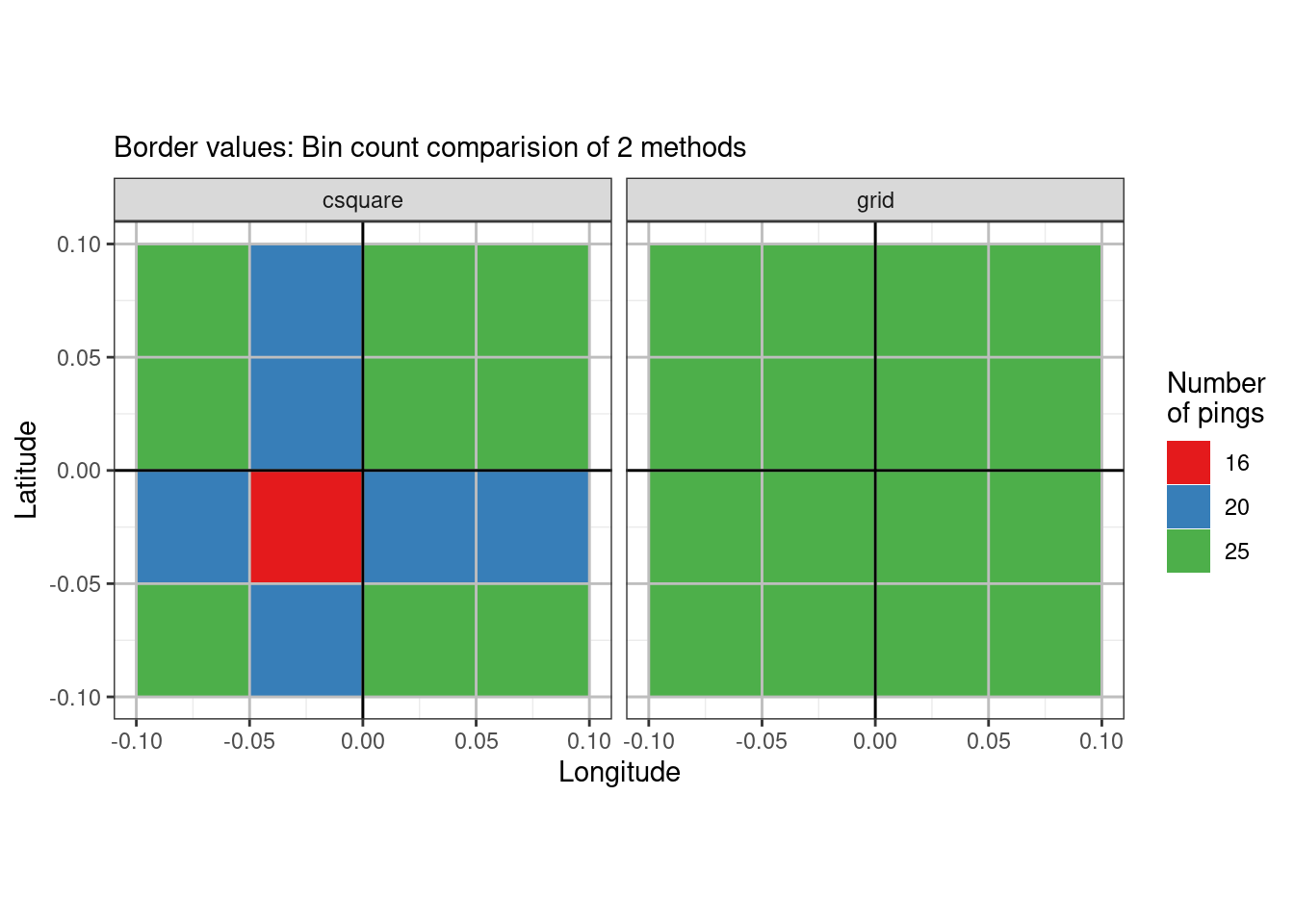
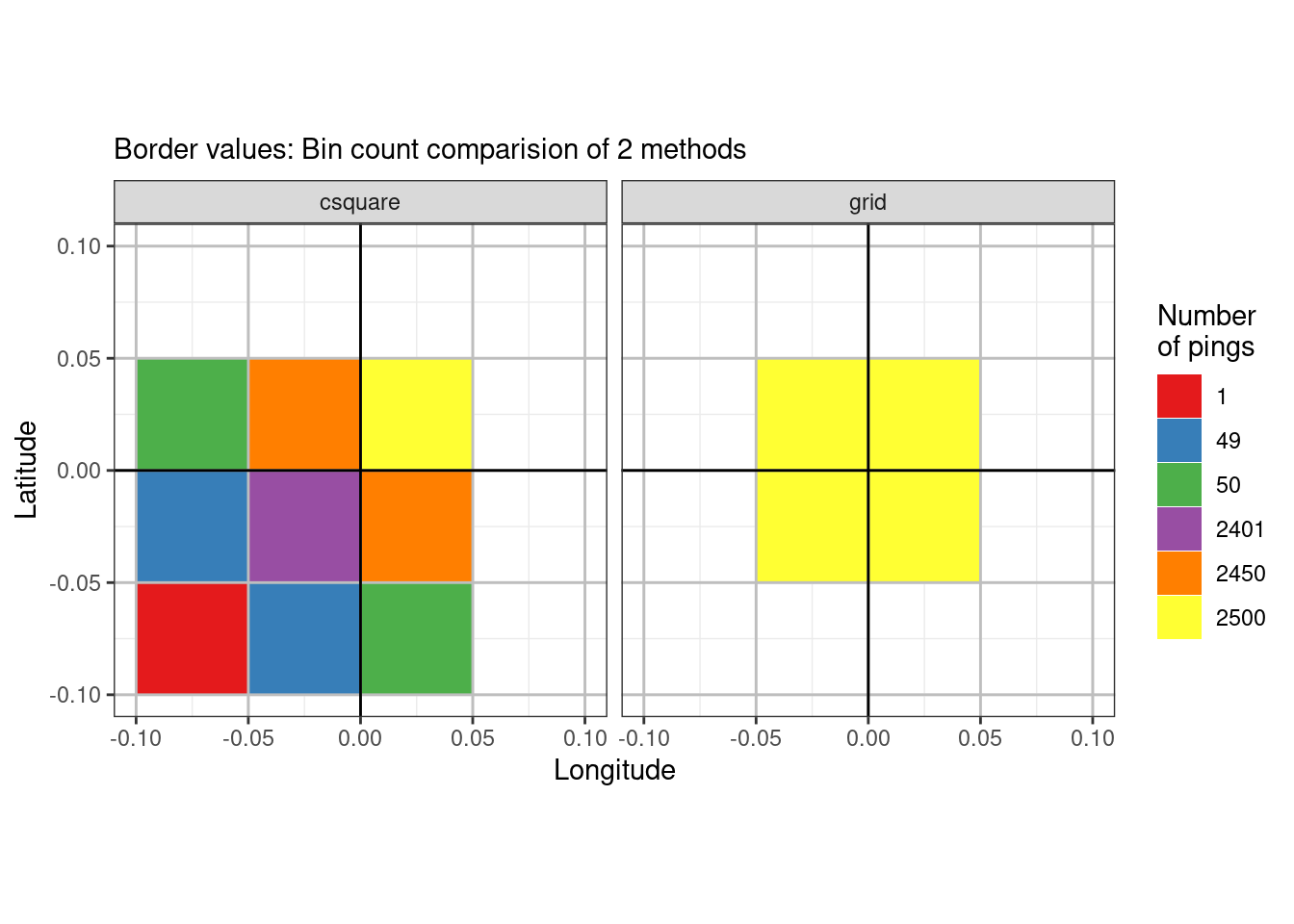
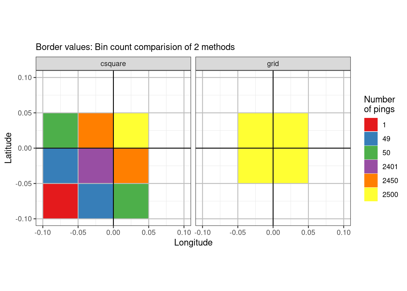
This post originated in that moi wanted to check if the code ‘x = lon %/% dx * dx + dx/2’ would give the same results as CSquare gridding as implemented in {vmstools}. Short answer is no. The former is more consistent, always resulting in binning such that if a value is exactly at ‘grid’-boundary it is included if on the lower boundary, excluded if on the upper boundary. In the {vmstools}-csquare case this depends on the global quarters. Now, somebody may argue that the practical consequences is miniscule and I would fully concur :-) Say so because a very small portion of real numeric data will be exactly on the grid boundary as focused on here. Leaving the devil in the details aside, the main message is that using ‘x = lon %/% dx * dx + dx/2’ is OK to use within R, arrow or duckdb code workflow. Why is this important? Because in the latter two workflows a csquare algorithm is not available/implemented.
code
rtip
Author

Einar Hjörleifsson

Published

June 18, 2025

Some synthetic data

library(tidyverse)
library(duckdbfs)
library(vmstools)
library(patchwork)

dx <- dy <- 0.05
g <- 
  expand_grid(lon = seq(-1, 1, by = 0.01),
              lat = seq(-1, 1, by = 0.01)) |> 
  mutate(cs = vmstools::CSquare(lon, lat, dx),
         x = lon %/% dx * dx + dx/2,
         y = lat %/% dy * dy + dy/2)
g <-
  bind_cols(g, vmstools::CSquare2LonLat(g$cs, dx)) |> 
  rename(lon2 = SI_LONG, lat2 = SI_LATI)
g |> glimpse()
Rows: 40,401
Columns: 7
$ lon  <dbl> -1, -1, -1, -1, -1, -1, -1, -1, -1, -1, -1, -1, -1, -1, -1, -1, -…
$ lat  <dbl> -1.00, -0.99, -0.98, -0.97, -0.96, -0.95, -0.94, -0.93, -0.92, -0…
$ cs   <chr> "5000:111:100:1", "5000:101:390:3", "5000:101:390:3", "5000:101:3…
$ x    <dbl> -0.975, -0.975, -0.975, -0.975, -0.975, -0.975, -0.975, -0.975, -…
$ y    <dbl> -0.975, -0.975, -0.975, -0.975, -0.975, -0.925, -0.925, -0.925, -…
$ lat2 <dbl> -1.0250121, -0.9750121, -0.9750121, -0.9750121, -0.9750121, -0.97…
$ lon2 <dbl> -1.025012, -1.025012, -1.025012, -1.025012, -1.025012, -1.025012,…
p <- 
  g |> 
  filter(between(lon, -0.125, 0.125),
         between(lat, -0.125, 0.125)) |> 
  ggplot() +
  theme_bw() +
  geom_hline(yintercept = 0, linewidth = 2, colour = "black") +
  geom_vline(xintercept = 0, linewidth = 2, colour = "black") +
  geom_vline(xintercept = seq(-0.1, 0.1, by = 0.05), colour = "grey") +
  geom_hline(yintercept = seq(-0.1, 0.1, by = 0.05), colour = "grey") +
  geom_point(aes(lon, lat), colour = "gold", size = 2) +
  labs(x = NULL, y = NULL) +
  coord_equal()
p1 <- 
  p +
  geom_segment(aes(x = lon, y = lat, xend = lon2, yend = lat2), colour = "blue") +
  geom_point(aes(lon2, lat2), colour = "blue", size = 4, shape = 1) +
  labs(subtitle = "C-Square")
p2 <-
  p +
  geom_segment(aes(x = lon, y = lat, xend = x, yend = y), colour = "red") +
  geom_point(aes(x, y), colour = "red", size = 4, shape = 1) +
  labs(subtitle = "Poor-man's grid")
p3 <-
  p +
  geom_segment(aes(x = lon, y = lat, xend = x, yend = y), colour = "red") +
  geom_segment(aes(x = lon, y = lat, xend = lon2, yend = lat2), colour = "blue") +
  geom_point(aes(x, y), colour = "red", size = 4, shape = 1) +
  geom_point(aes(lon2, lat2), colour = "blue", size = 4, shape = 1) +
  labs(subtitle = "Both")
p1 + p2

p3

Some counts

bind_rows(g |> select(lon = x, lat = y) |> mutate(what = "grid"),
          g |> select(lon = lon2, lat = lat2) |> mutate(what = "csquare")) |> 
  mutate(lon = round(lon, 4),
         lat = round(lat, 4)) |> 
  count(what, lon, lat) |> 
  filter(between(lon, -0.1, 0.1),
         between(lat, -0.1, 0.1)) |> 
  ggplot() +
  theme_bw() +
  geom_tile(aes(lon, lat, fill = factor(n))) +
  geom_vline(xintercept = seq(-0.1, 0.1, by = 0.05), colour = "grey") +
  geom_hline(yintercept = seq(-0.1, 0.1, by = 0.05), colour = "grey") +
  geom_hline(yintercept = 0) +
  geom_vline(xintercept = 0) +
  facet_wrap(~ what) +
  labs(x = "Longitude", y = "Latitude", fill = "Number\nof pings",
       subtitle = "Border values: Bin count comparision of 2 methods") +
  scale_fill_brewer(palette = "Set1") +
  coord_equal()

Another view

g <- 
  expand_grid(lon = seq(-0.05, 0.0499, by = 0.001),
            lat = seq(-0.05, 0.0499, by = 0.001)) |> 
  mutate(cs = vmstools::CSquare(lon, lat, dx),
         x = lon %/% dx * dx + dx/2,
         y = lat %/% dy * dy + dy/2)
g <-
  bind_cols(g, vmstools::CSquare2LonLat(g$cs, dx)) |> 
  rename(lon2 = SI_LONG, lat2 = SI_LATI)
bind_rows(g |> select(lon = x, lat = y) |> mutate(what = "grid"),
          g |> select(lon = lon2, lat = lat2) |> mutate(what = "csquare")) |> 
  mutate(lon = round(lon, 4),
         lat = round(lat, 4)) |> 
  count(what, lon, lat) |> 
  filter(between(lon, -0.1, 0.1),
         between(lat, -0.1, 0.1)) |> 
  ggplot() +
  theme_bw() +
  geom_tile(aes(lon, lat, fill = factor(n))) +
  geom_vline(xintercept = seq(-0.1, 0.1, by = 0.05), colour = "grey") +
  geom_hline(yintercept = seq(-0.1, 0.1, by = 0.05), colour = "grey") +
  geom_hline(yintercept = 0) +
  geom_vline(xintercept = 0) +
  facet_wrap(~ what) +
  labs(x = "Longitude", y = "Latitude", fill = "Number\nof pings",
       subtitle = "Border values: Bin count comparision of 2 methods") +
  scale_fill_brewer(palette = "Set1") +
  coord_equal()

Some additional dissections

The R convention:

expand_grid(lon = seq(-0.05, 0.0499, by = 0.001),
            lat = seq(-0.05, 0.0499, by = 0.001)) |> 
  mutate(lon = santoku::chop(lon, breaks = seq(-0.1, 0.1, by = 0.05)),
         lat = santoku::chop(lat, breaks = seq(-0.1, 0.1, by = 0.05))) |> 
  count(lon, lat)
# A tibble: 4 × 3
  lon        lat            n
  <fct>      <fct>      <int>
1 [-0.05, 0) [-0.05, 0)  2500
2 [-0.05, 0) [0, 0.05)   2500
3 [0, 0.05)  [-0.05, 0)  2500
4 [0, 0.05)  [0, 0.05)   2500

Moi:

dx <- 0.05
expand_grid(lon = seq(-0.05, 0.0499, by = 0.001),
            lat = seq(-0.05, 0.0499, by = 0.001)) |> 
  mutate(lon = lon %/% dx * dx + dx/2,
         lat = lat %/% dy * dy + dy/2) |> 
  count(lon, lat)
# A tibble: 4 × 3
     lon    lat     n
   <dbl>  <dbl> <int>
1 -0.025 -0.025  2500
2 -0.025  0.025  2500
3  0.025 -0.025  2500
4  0.025  0.025  2500

CSquare:

dx <- 0.05
expand_grid(lon = seq(-0.05, 0.0499, by = 0.001),
            lat = seq(-0.05, 0.0499, by = 0.001)) |> 
  mutate(cs = vmstools::CSquare(lon, lat, dx),
         lon = vmstools::CSquare2LonLat(cs, dx)$SI_LONG,
         lat = vmstools::CSquare2LonLat(cs, dx)$SI_LATI) |> 
  count(lon, lat)
# A tibble: 9 × 3
      lon     lat     n
    <dbl>   <dbl> <int>
1 -0.0750 -0.0750     1
2 -0.0750 -0.0250    49
3 -0.0750  0.0250    50
4 -0.0250 -0.0750    49
5 -0.0250 -0.0250  2401
6 -0.0250  0.0250  2450
7  0.0250 -0.0750    50
8  0.0250 -0.0250  2450
9  0.0250  0.0250  2500