library(terra)
library(tidyterra)
library(sf)
library(tidyverse)
library(patchwork)
The data
To answer the question we use three different data sources:
- A GEBCO raster that contains the depth information
- The Icelandic EEZ, as a polygon
- The island itself, as a polygon
# Data -------------------------------------------------------------------------
# Gebco data obtained from: https://download.gebco.net
r <- rast(here::here("data-raw/depth/GEBCO_05_Jun_2025_14e882e0ff28/gebco_2024_n73.3887_s51.2402_w-36.8262_e-1.8457.tif"))
iceland <-
  read_sf("ftp://ftp.hafro.is/pub/data/shapes/iceland_coastline.gpkg") %>%
  st_transform(crs = 4326)
eez <-
  read_sf("ftp://ftp.hafro.is/pub/data/shapes/eez_iceland.gpkg")
# limit gebco data to the eez bounding box
r <- crop(r, eez)
p1 <-
  ggplot() +
  theme_void() +
  tidyterra::geom_spatraster(data = r) +
  scale_fill_viridis_c() +
  labs(subtitle = "The GEBCO raster") +
  theme(legend.position = "none")
p2 <-
  p1 +
  geom_sf(data = eez  |> st_cast("MULTILINESTRING"),
          colour = "white") +
  labs(subtitle = "add eez")
p3 <-
  p2 +
  geom_sf(data = iceland, fill = "grey") +
  labs(subtitle = "add iceland")
p1 + p2 + p3 + plot_layout(guides = "collect")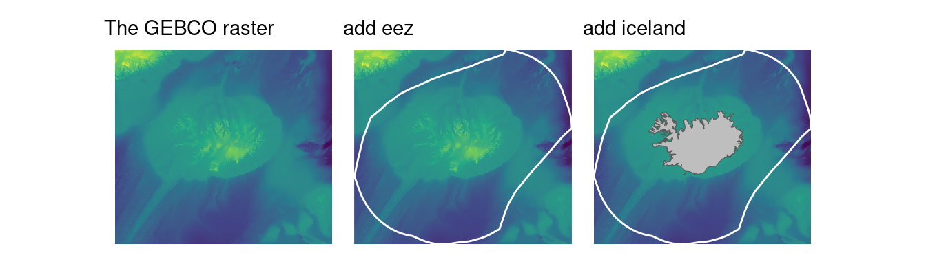
Spatial processing
The first objective is to limit the GEBCO raster grid only to area within the EEZ but excluding the data above sea-level. The steps are:
- Create a proper EEZ polygon that excludes the island
- “Remove” all grid points outside the above area. This is called masking in raster-lingo.
# step 1
eez <-
  eez |>
  st_difference(iceland) %>%
  mutate(area = lwgeom::st_geod_area(.)) %>%
  select(area)
# step 2
r_eez <- mask(r, eez)
# some extra filtering of positive elevations
i <- values(r_eez) > 0
values(r_eez)[i] <- NA
ggplot() +
  theme_void() +
  geom_spatraster(data = r_eez) +
  scale_fill_viridis_c() +
  theme(legend.position = "none") +
  geom_spatraster_contour(data = r_eez,
                          breaks = c(-1000, -500, -250),
                          colour = "black") +
  labs(subtitle = "The masked GEBCO raster",
       caption = "Contours: 250, 500 and 1000 meter depth rasters")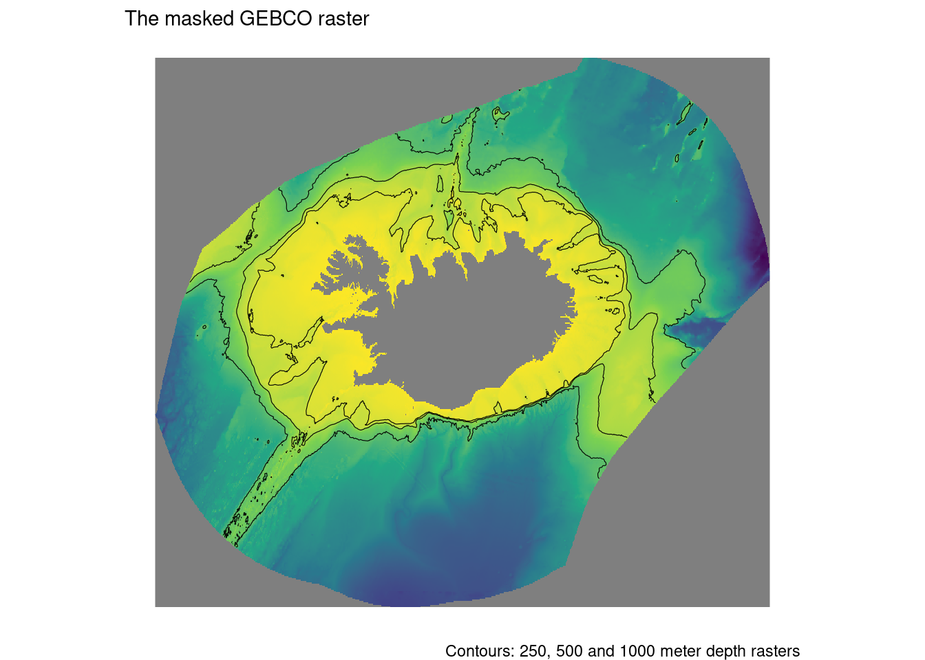
Area calculations
Now the question was how many square kilometers of the EEZ was below 1000 meters depth. Since we are at it, we may as well try to expand the analysis to calculate the area deeper than every 100 meters. The steps are as follows:
- Get the depth value for each grid point
- Calculate the area of each 100 meter depth range, here using a (hopefully) understandable loop.
# Step 1
v <- values(r_eez) |> as.vector()
# Step 2
zs <- seq(-3000, 0, by = 100)
res <- list()
for(z in 1:length(zs)) {
  i <- v > zs[z]
  r_tmp <- r_eez
  r_tmp[i] <- NA
  res[[z]] <- expanse(r_tmp)
}
names(res) <- zs
d <-
  bind_rows(res, .id = "depth") |>
  mutate(depth = as.numeric(depth),
         area_kkm2 = round(area / 1e9)) |>
  select(depth, area_kkm2) |>
  mutate(percentage = round(area_kkm2 / max(area_kkm2) * 100))
d |>
  ggplot(aes(-depth, area_kkm2)) +
  geom_point(size = 1) +
  geom_line() +
  expand_limits(y = 0) +
  scale_x_continuous(breaks = seq(0, 3000, by = 200)) +
  scale_y_continuous(breaks = seq(0, 800, by = 100)) +
  labs(x = "Depth more than specified [meters]",
       y = "Area [thousand square kilometers")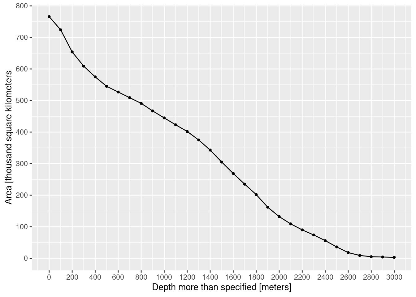
d |>
  mutate(Depth = -depth) |>
  arrange(-depth) |>
  mutate(shallower = 100 - percentage) |>
  select(Depth, 'Area deeper [kkm2]' = area_kkm2, 'Deeper [%]' = percentage, 'Shallower [%]' = shallower) |>
knitr::kable(caption = "Area of depth greater than specified within the Icelandic EEZ and percentage deeper and shallower.")| Depth | Area deeper [kkm2] | Deeper [%] | Shallower [%] |
|---|---|---|---|
| 0 | 766 | 100 | 0 |
| 100 | 724 | 95 | 5 |
| 200 | 654 | 85 | 15 |
| 300 | 609 | 80 | 20 |
| 400 | 575 | 75 | 25 |
| 500 | 545 | 71 | 29 |
| 600 | 527 | 69 | 31 |
| 700 | 509 | 66 | 34 |
| 800 | 491 | 64 | 36 |
| 900 | 467 | 61 | 39 |
| 1000 | 445 | 58 | 42 |
| 1100 | 423 | 55 | 45 |
| 1200 | 402 | 52 | 48 |
| 1300 | 375 | 49 | 51 |
| 1400 | 343 | 45 | 55 |
| 1500 | 305 | 40 | 60 |
| 1600 | 269 | 35 | 65 |
| 1700 | 235 | 31 | 69 |
| 1800 | 202 | 26 | 74 |
| 1900 | 162 | 21 | 79 |
| 2000 | 132 | 17 | 83 |
| 2100 | 109 | 14 | 86 |
| 2200 | 90 | 12 | 88 |
| 2300 | 74 | 10 | 90 |
| 2400 | 56 | 7 | 93 |
| 2500 | 36 | 5 | 95 |
| 2600 | 18 | 2 | 98 |
| 2700 | 9 | 1 | 99 |
| 2800 | 5 | 1 | 99 |
| 2900 | 4 | 1 | 99 |
| 3000 | 3 | 0 | 100 |
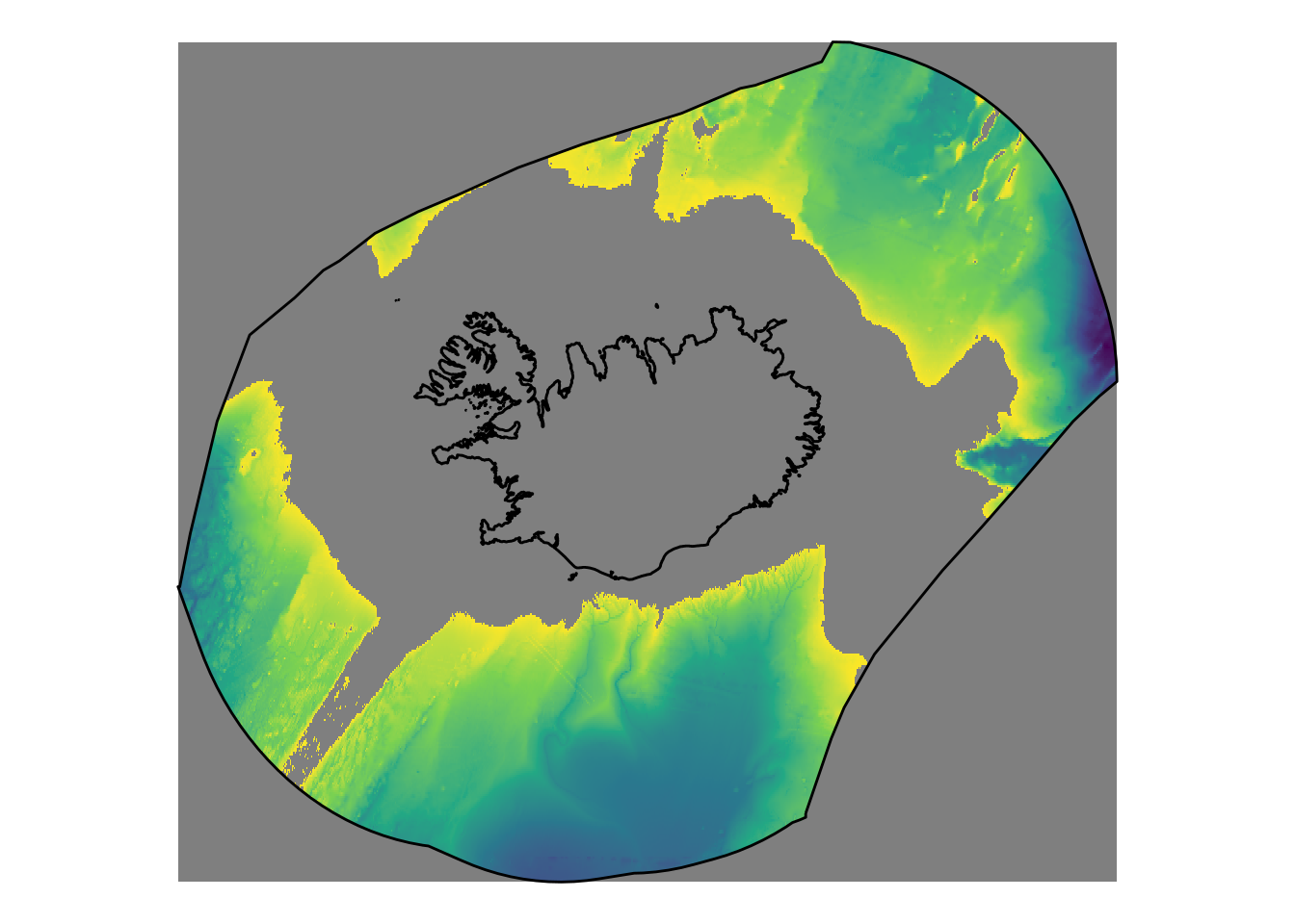
The answer
So according the above data and analysis the total EEZ is 766 thousand \(km^2\). The area deeper than 1000 meter depth is 445 thousand \(km^2\), that being 58% of the total EEZ. Spatially this area looks something like this:
v <- values(r_eez) |> as.vector()
i <- v >= -1000
r_eez[i] <- NA
ggplot() +
  theme_void() +
  tidyterra::geom_spatraster(data = r_eez) +
  geom_sf(data = eez |> st_cast("MULTILINESTRING")) +
  scale_fill_viridis_c() +
  theme(legend.position = "none")