Transformation
Tidy dataframes
The defintion of a tidy dataset:
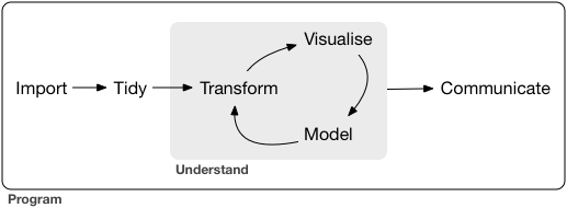
Each column is a variable, and each row is an observation.Having a tidy dataset is fundamental in the tidyverse code-flow:
Tidy datasets are all alike but every messy dataset is messy in its own way.
- Hadley Wickham- Although you can work (read: code) starting off with an untidy dataset you will soon hit troubles
- In fisheries science we tend to have very similar variables across different types of data:
- Landings monitoring (full census or sampled based)
- Fishermen’s logbooks
- Scientific fisheries resource surveys (trawl, accoustic, UV, …)
- Continuous positioning data (AIS, VMS, GIS)
- If we have similar structures we may in the end be able to use very similar code-flow to explore, transform and vizualize different datasets.
Excercise
Group discussion: What common variables may we be measuring in the data-sets mentioned above.
An untidy version of the Icelandic bottom trawl survey can be read in via:
library(tidyverse)
sur <-
  read_csv("ftp://ftp.hafro.is/pub/data/csv/is_smb.csv")
glimpse(sur)
Rows: 19,846
Columns: 40
$ id <dbl> 44929, 44928, 44927, 44926, 44925, 44922, 44921, 44920,…
$ date <date> 1990-03-16, 1990-03-16, 1990-03-16, 1990-03-16, 1990-0…
$ year <dbl> 1990, 1990, 1990, 1990, 1990, 1990, 1990, 1990, 1990, 1…
$ vid <dbl> 1307, 1307, 1307, 1307, 1307, 1307, 1307, 1307, 1307, 1…
$ tow_id <chr> "670-15", "670-13", "670-12", "670-1", "670-2", "720-1"…
$ t1 <dttm> 1990-03-16 05:05:00, 1990-03-16 07:48:00, 1990-03-16 0…
$ t2 <dttm> 1990-03-16 06:05:00, 1990-03-16 08:51:00, 1990-03-16 1…
$ lon1 <dbl> -20.70367, -20.49767, -20.44650, -20.21500, -19.99100, …
$ lat1 <dbl> 66.52250, 66.50917, 66.58583, 66.57417, 66.65767, 67.24…
$ lon2 <dbl> -20.73167, -20.53350, -20.29083, -20.07750, -19.98883, …
$ lat2 <dbl> 66.59167, 66.57583, 66.61550, 66.61600, 66.72383, 67.29…
$ ir <chr> "62C9", "62C9", "62C9", "62C9", "62D0", "63C9", "63C9",…
$ ir_lon <dbl> -20.5, -20.5, -20.5, -20.5, -19.5, -20.5, -20.5, -20.5,…
$ ir_lat <dbl> 66.75, 66.75, 66.75, 66.75, 66.75, 67.25, 67.25, 67.25,…
$ z1 <dbl> 297, 302, 205, 88, 129, 249, 332, 244, 291, 230, 140, 3…
$ z2 <dbl> 330, 314, 291, 117, 172, 307, 360, 256, 282, 270, 158, …
$ temp_s <dbl> 1.1, 1.1, 1.0, 1.1, 0.9, 1.3, 1.2, 1.2, 1.1, 1.0, 1.0, …
$ temp_b <dbl> NA, 1.0, NA, 1.0, 1.1, 1.0, -0.5, 0.9, 0.9, 0.9, NA, -0…
$ speed <dbl> 4.0, 3.8, 3.2, 4.0, 4.1, 4.1, 3.9, 3.8, 3.9, 3.9, 4.0, …
$ duration <dbl> 60, 63, 74, 60, 59, 59, 61, 64, 62, 62, 60, 59, 65, 66,…
$ towlength <dbl> 4, 4, 4, 4, 4, 4, 4, 4, 4, 4, 4, 4, 4, 4, 4, 4, 4, 3, 4…
$ horizontal <dbl> NA, NA, NA, NA, NA, NA, NA, NA, NA, NA, NA, NA, NA, NA,…
$ verical <dbl> 2.0, 3.0, 2.4, 2.6, NA, NA, NA, 2.2, 2.0, 2.0, 2.0, 2.8…
$ wind <dbl> 15, 15, 15, 15, 12, 9, 9, 7, 7, 5, 5, 3, 7, 7, 1, 7, 7,…
$ wind_direction <dbl> 5, 5, 5, 9, 9, 9, 9, 9, 9, 14, 14, 5, 5, 5, 32, 36, 5, …
$ bormicon <dbl> 3, 3, 3, 3, 3, 3, 3, 3, 3, 3, 3, 3, 3, 3, 3, 3, 3, 3, 2…
$ oldstrata <dbl> 34, 34, 34, 34, 34, 33, 36, 33, 33, 34, 34, 34, 34, 41,…
$ newstrata <dbl> 31, 31, 31, 32, 32, 18, 37, 18, 18, 31, 32, 31, 31, 36,…
$ cod_kg <dbl> 56.30017, 29.28811, 34.62728, 8.32594, 43.83642, 1.2309…
$ cod_n <dbl> 155, 75, 125, 13, 81, 6, 0, 3, 0, 52, 330, 77, 30, 48, …
$ haddock_kg <dbl> 0.50302238, 0.00000000, 0.46842356, 2.39978621, 11.5888…
$ haddock_n <dbl> 16, 0, 17, 7, 42, 0, 0, 0, 0, 12, 10, 0, 0, 0, 0, 0, 1,…
$ saithe_kg <dbl> 0.00, 0.00, 0.00, 0.00, 0.00, 0.00, 0.00, 0.00, 0.00, 0…
$ saithe_n <dbl> 0, 0, 0, 0, 0, 0, 0, 0, 0, 0, 0, 0, 0, 0, 0, 0, 0, 5893…
$ wolffish_kg <dbl> 4.7770270, 3.1999367, 1.7183545, 8.4568957, 11.6068288,…
$ wolffish_n <dbl> 12, 1, 2, 27, 26, 0, 0, 0, 0, 2, 69, 0, 0, 27, 0, 0, 29…
$ plaice_kg <dbl> 0.0000000, 0.0000000, 0.3660489, 4.2098115, 2.4292287, …
$ plaice_n <dbl> 0, 0, 1, 6, 3, 0, 0, 0, 0, 0, 1, 0, 0, 0, 0, 0, 0, 0, 0…
$ monkfish_kg <dbl> 0, 0, 0, 0, 0, 0, 0, 0, 0, 0, 0, 0, 0, 0, 0, 0, 0, 0, 0…
$ monkfish_n <dbl> 0, 0, 0, 0, 0, 0, 0, 0, 0, 0, 0, 0, 0, 0, 0, 0, 0, 0, 0…If you are working in Excel this wide format is very common. Lets isolate the biological variables but also retain the station id:
wide <-
  sur |>
  select(id, cod_kg:monkfish_n)
wide |> glimpse()
Rows: 19,846
Columns: 13
$ id <dbl> 44929, 44928, 44927, 44926, 44925, 44922, 44921, 44920, 44…
$ cod_kg <dbl> 56.30017, 29.28811, 34.62728, 8.32594, 43.83642, 1.23096, …
$ cod_n <dbl> 155, 75, 125, 13, 81, 6, 0, 3, 0, 52, 330, 77, 30, 48, 13,…
$ haddock_kg <dbl> 0.50302238, 0.00000000, 0.46842356, 2.39978621, 11.5888963…
$ haddock_n <dbl> 16, 0, 17, 7, 42, 0, 0, 0, 0, 12, 10, 0, 0, 0, 0, 0, 1, 20…
$ saithe_kg <dbl> 0.00, 0.00, 0.00, 0.00, 0.00, 0.00, 0.00, 0.00, 0.00, 0.00…
$ saithe_n <dbl> 0, 0, 0, 0, 0, 0, 0, 0, 0, 0, 0, 0, 0, 0, 0, 0, 0, 5893, 0…
$ wolffish_kg <dbl> 4.7770270, 3.1999367, 1.7183545, 8.4568957, 11.6068288, 0.…
$ wolffish_n <dbl> 12, 1, 2, 27, 26, 0, 0, 0, 0, 2, 69, 0, 0, 27, 0, 0, 29, 6…
$ plaice_kg <dbl> 0.0000000, 0.0000000, 0.3660489, 4.2098115, 2.4292287, 0.0…
$ plaice_n <dbl> 0, 0, 1, 6, 3, 0, 0, 0, 0, 0, 1, 0, 0, 0, 0, 0, 0, 0, 0, 0…
$ monkfish_kg <dbl> 0, 0, 0, 0, 0, 0, 0, 0, 0, 0, 0, 0, 0, 0, 0, 0, 0, 0, 0, 0…
$ monkfish_n <dbl> 0, 0, 0, 0, 0, 0, 0, 0, 0, 0, 0, 0, 0, 0, 0, 0, 0, 0, 0, 0…
Excercise
- Identify the variables in the wide data frame
- Identify the measurements in the wide data frame
pivot_longer
To make a wide table longer, we can employ the pivot_longer-function. Lets first focus just on the abundance measurments:
long <-
  wide %>%
  # select just the abundance variables
  select(id, ends_with("_n")) %>%
  pivot_longer(cols = -id, names_to = "species", values_to = "n") %>%
  mutate(species = str_remove(species, "_n"))
glimpse(long)
Rows: 119,076
Columns: 3
$ id <dbl> 44929, 44929, 44929, 44929, 44929, 44929, 44928, 44928, 44928,…
$ species <chr> "cod", "haddock", "saithe", "wolffish", "plaice", "monkfish", …
$ n <dbl> 155, 16, 0, 12, 0, 0, 75, 0, 0, 1, 0, 0, 125, 17, 0, 2, 1, 0, …So we have moved from a dataframe that was 19846 rows with 7 columns to a dataframe of 119076 (19846 stations x 6 species) rows with only 3 columns, each being a variable:
- id: Station id
- species: Species name
- n: Abundance (standardized to 4 nautical miles)
This latter (longer) format is the proper format for efficient computer programming. The following exercise should illustrate that.
Excercise
- Use the wide-dataframe above and write a code to calculate the median abundance (***_n column) for each species
- Use the long-dataframe above and write a code to calculate the median abundance for each species
- Ammend the long-dataframe code to include min, max and mean abundance.
- Would you like to try adding the calculation of the min, max and mean on the wide-dataframe (item 1 above)?
Solution:
wide %>%
  summarise(cod = median(cod_n),
            haddock = median(haddock_n),
            saithe = median(saithe_n),
            wolfish = median(wolffish_n),
            plaice = median(plaice_n),
            monkfish = median(monkfish_n))
long %>%
  group_by(species) %>%
  summarise(median = median(n),
            mean = mean(n),
            min = min(n),
            max = max(n))
pivot_wider
When reconstructing untidy tables we sometimes may need to make a long table wider again. We may actually also want to make long table wider in our communications.
In the above example we only made a long table for abundance (n). We could modify the above code for the biomass (kg). Doing all in one step requires the use of pivot_wider, the steps being:
- Make a table containing id, current variable (cod_n, cod_kg, …) and the corresponding value (abundance or biomass)
- Separate the value measured (kg or n) from the species name
- Generate separate columns for abundance (n) and biomass (kg)
long <-
  wide %>%
  # step 1
  pivot_longer(-id) %>%
  # step 2
  separate(name, sep = "_", into = c("species", "variable")) %>%
  # step 3
  pivot_wider(names_from = variable, values_from = value)
Excercise
- Run each code step above on the wide-table and observe the results:
step1 <- wide |> pivot_longer(-id)
glimpse(step1)
step2 <- step1 |> separate(name, sep = "_", into = c("species", "variable"))
glimpse(step2)
step3 <- step2 |> pivot_wider(names_from = variable)
glimpse(step3)
Further reading
As said above “every messy dataset is messy in its own way”. This means that it is difficult to generalize how to tidy e.g. your data (if they are untidy). In the r4ds book there are good general chapter (Data tidying) that may help you along your own path towards tidyness.