Statistical Modelling with R
One has a data set with some variables of interest (length, weight, catch etc.) How do we go about analyzing this?
Step 1: Descriptive statistics
We start off with data exploration, visualization and summarize data in a meaningful way. This is something we have covered in the visualization and transformation modules above.
Spatial maps are appealing provided one has spatial data (e.g. latitude and longitude values of stations).
Some useful pointers when exploring your data set:
For Discrete variable - Pie charts / Bar Graphs (usually better). All categorical variables are discrete and some numerical variables e.g., numbers of fish. One counts discrete data (e.g. 20 fish).
For Continuous variables - histograms, scatterplots, boxplots are more appropriate. Continuous means when a numerical variable can have any numerical value on some intervals. One measures continuous data (e.g., length is measured as 13.46cm).
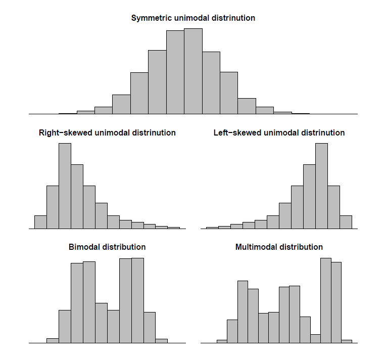
Distribution shapes
There are different shapes of distribution one should be aware of when plotting the data because this can affect the choice of statistic to be used. If the distribution is skewed, bimodal or multimodal the median shall be used rather then the mean. The median should also be preferred if there are outliers in the measurement.
When distributions are skewed, data can be transformed to achieve normality using log or sqrt.
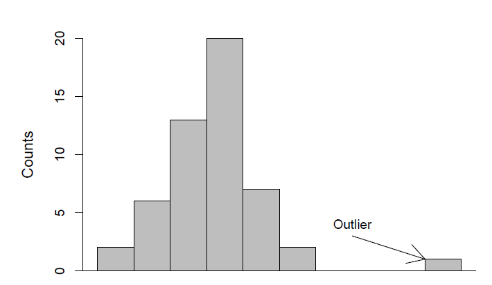
Outliers
Outliers are measurements that differ greatly from other measurements in the sample. Important to look at them specifically and consider their cause. They can be identified during the data exploration process.
Missing values
NAs were briefly introduced in the transformation module. NAs are not the same as zeros! It indicates missingness of data, meaning it was not measured. It is important to remove or replace NAs before calculating data summaries.
Statistics that describe central tendency and spread
Measures of central tendency were introduced in the transformation module i.e. mean, median. In addition, we would like to know the spread of the data. These statistics describe how spread out the measurements are.
Range: obtained by \(x_{max} - x_{min}\)
Quartile: There are three quartiles
include_graphics("images/quartiles.png")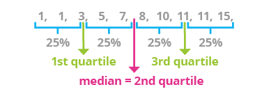
Interquartile range: \(Q_3 - Q_1\)
Five number summary: is informative for skewed distributions
min, Q_1, Q_2, Q_3, max
w <-
  read_csv("ftp://ftp.hafro.is/pub/data/csv/minke.csv")

w %>% summary()
id date lon
Min. : 1 Min. :2003-08-18 17:00:00.00 Min. :-24.63
1st Qu.: 1503 1st Qu.:2004-06-22 03:00:00.00 1st Qu.:-22.75
Median :20677 Median :2006-01-16 13:00:00.00 Median :-20.94
Mean :14547 Mean :2005-09-26 08:10:44.21 Mean :-19.69
3rd Qu.:20982 3rd Qu.:2006-08-14 11:30:00.00 3rd Qu.:-16.43
Max. :21072 Max. :2007-09-02 16:00:00.00 Max. :-13.21
lat area length weight
Min. :63.30 Length:190 Min. :461.0 Min. :1663
1st Qu.:64.17 Class :character 1st Qu.:725.5 1st Qu.:3462
Median :65.13 Mode :character Median :770.0 Median :4165
Mean :65.11 Mean :752.6 Mean :4084
3rd Qu.:66.10 3rd Qu.:802.8 3rd Qu.:4620
Max. :67.04 Max. :871.0 Max. :5685
NA's :169
age sex maturity stomach.volume
Min. : 3.40 Length:190 Length:190 Min. : 0.00
1st Qu.:11.40 Class :character Class :character 1st Qu.: 14.75
Median :17.30 Mode :character Mode :character Median : 32.00
Mean :18.97 Mean : 41.91
3rd Qu.:24.30 3rd Qu.: 57.25
Max. :47.40 Max. :200.00
NA's :17 NA's :2
stomach.weight year
Min. : 0.000 Min. :2003
1st Qu.: 2.312 1st Qu.:2004
Median : 7.819 Median :2006
Mean : 14.822 Mean :2005
3rd Qu.: 17.483 3rd Qu.:2006
Max. :106.250 Max. :2007
NA's :2 summary(w) id date lon
Min. : 1 Min. :2003-08-18 17:00:00.00 Min. :-24.63
1st Qu.: 1503 1st Qu.:2004-06-22 03:00:00.00 1st Qu.:-22.75
Median :20677 Median :2006-01-16 13:00:00.00 Median :-20.94
Mean :14547 Mean :2005-09-26 08:10:44.21 Mean :-19.69
3rd Qu.:20982 3rd Qu.:2006-08-14 11:30:00.00 3rd Qu.:-16.43
Max. :21072 Max. :2007-09-02 16:00:00.00 Max. :-13.21
lat area length weight
Min. :63.30 Length:190 Min. :461.0 Min. :1663
1st Qu.:64.17 Class :character 1st Qu.:725.5 1st Qu.:3462
Median :65.13 Mode :character Median :770.0 Median :4165
Mean :65.11 Mean :752.6 Mean :4084
3rd Qu.:66.10 3rd Qu.:802.8 3rd Qu.:4620
Max. :67.04 Max. :871.0 Max. :5685
NA's :169
age sex maturity stomach.volume
Min. : 3.40 Length:190 Length:190 Min. : 0.00
1st Qu.:11.40 Class :character Class :character 1st Qu.: 14.75
Median :17.30 Mode :character Mode :character Median : 32.00
Mean :18.97 Mean : 41.91
3rd Qu.:24.30 3rd Qu.: 57.25
Max. :47.40 Max. :200.00
NA's :17 NA's :2
stomach.weight year
Min. : 0.000 Min. :2003
1st Qu.: 2.312 1st Qu.:2004
Median : 7.819 Median :2006
Mean : 14.822 Mean :2005
3rd Qu.: 17.483 3rd Qu.:2006
Max. :106.250 Max. :2007
NA's :2 w %>% select(age) %>% summary() age
Min. : 3.40
1st Qu.:11.40
Median :17.30
Mean :18.97
3rd Qu.:24.30
Max. :47.40
NA's :17 Variance \(s^2\): a measure of dispersion around the mean
Standard deviation \(s\): square root of variance
Standard error - \(se\):
s/sqrt(n)
Descriptive analysis describes the characteristics of a data set and can summarize based on groups in the data but conclusions are not drawn beyond the data we have.
Step 2 - Inferential Statistics
Inferential statistics are techniques that allow us to use the sample to generalize to the population or make inferences about the population. Sample should be an accurate representation of the population.
Population and Sample
Sample - the set of subjects that are sampled from a given population (e.g., landed catch samples from landing sites)
Population - the set of all subjects that inference should be made about (e.g., skipjack tuna population in Saint Lucian waters)
Our data is almost always a sample
Types of inferential statistics
Regression Analysis and hypothesis testing are examples of inferential statistics.
Regression models show the relationship between your dependent variable (response variable Y) and a set of independent variables (explanatory variable X). This statistical method lets you predict the value of the dependent variable based on different values of the independent variables. Hypothesis tests are incorporated in this procedure to determine whether the relationships observed in sample data actually exist in the data set.
The ideology behind hypothesis tests
A hypothesis is formed \(H_1\) which describes what we want to demonstrate (e.g. there is a difference in length between the different sexes of minke whales) and another that describes a null \(H_0\) case (e.g. there is no difference.
A statistic is found that has a known probabiliy distribution. It is defined what values of the test statistics are “improbable” according to the probability distribution in the null case.
If the retrieved estimate classifies as “improbable” the hypothesis for the null case is rejected and the alternate hypothesis is claimed (use \(p\)-value to decide).
Those who would like to learn more about these concepts can use statistics resources available online:
Linear Models
Statistical Models
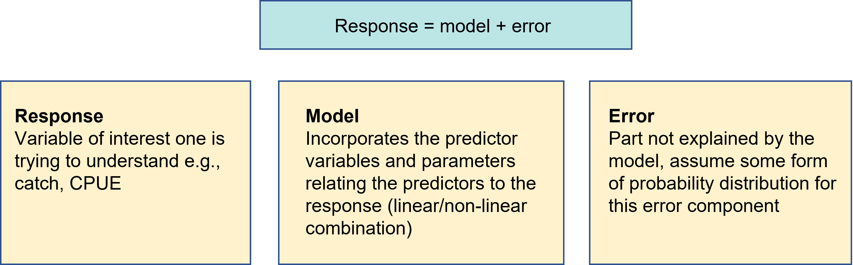
Purpose
- Fit our model to our observed data
- This fitting is an estimation procedure
- To describe the relationship between \(Y\) and \(X\)
- To determine how much of the variation (uncertainty) in \(Y\) can be explained by the relationship with \(X\) and how much is unexplained (error)
- To predict new values of \(Y\) from new values of \(X\)
- The modelling procedure can help us decide which models give the best fit to our observed sample data
- Model diagnostics is important to ensure the model is adequate
What does ‘linear’ mean?
The term linear model is used in two distinct ways.
First, a model of a straight line relationship (most common)
Second, a model in which any variable of interest (\(y\)) is described by a linear combination of a series of parameters. The regression function is linear. Now linear refers to a combination of parameters not the shape of the relationship.
Using the second definition linear models can represent not only straight line relationships but also curvilinear relationships such as the models with polynomial terms.
Linear Models
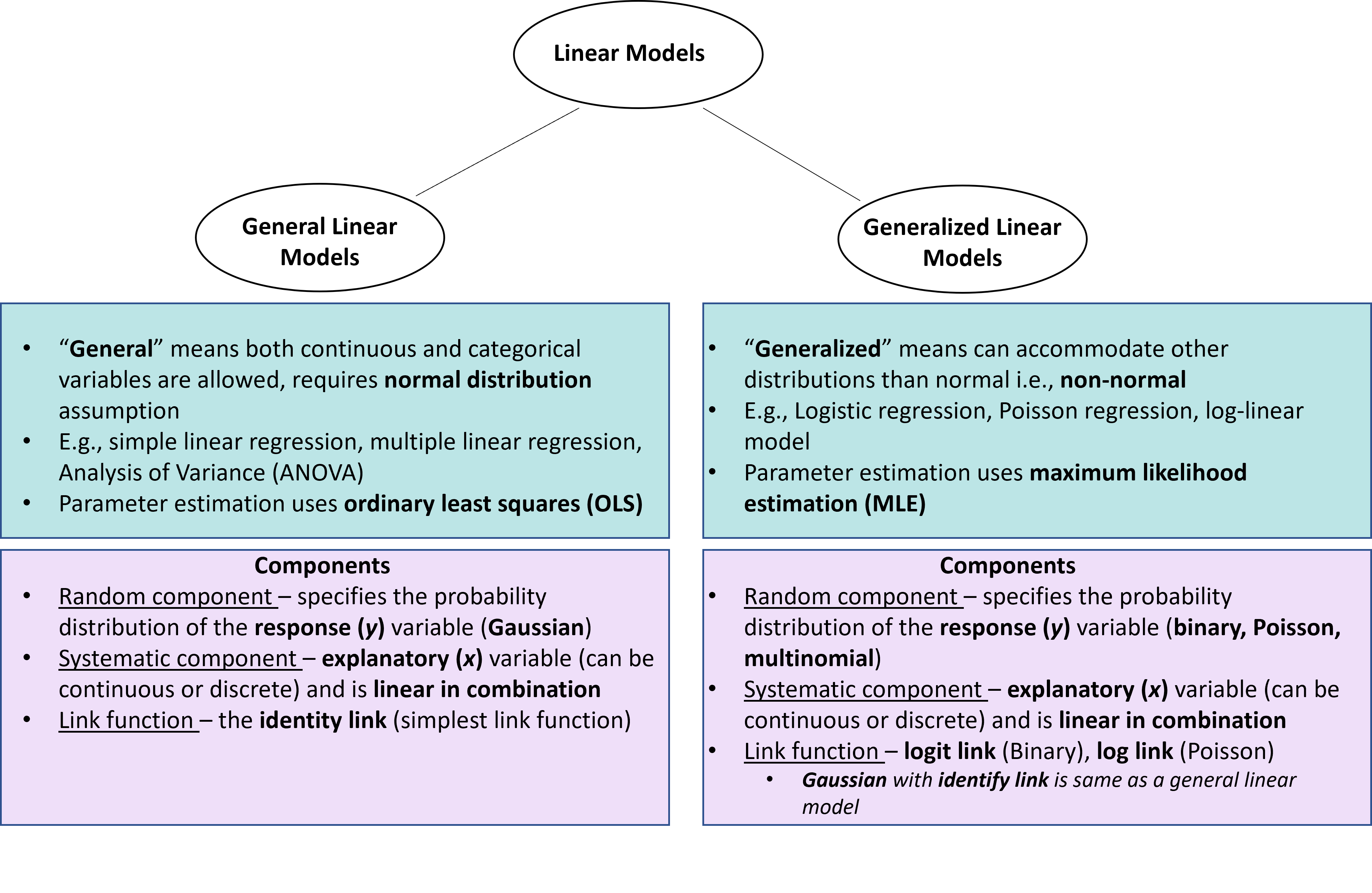
Simple linear model (Linear Regression)
Model formulation:
\[Y = \beta_0 + \beta_1X + \epsilon \] where:
- Y is the response variable
- \(\beta_0\) and \(\beta_1\) are parameters to be estimated
- \(\epsilon\) is the error term that assumes normal distribution with mean 0 and standard deviation \(\sigma^2\)
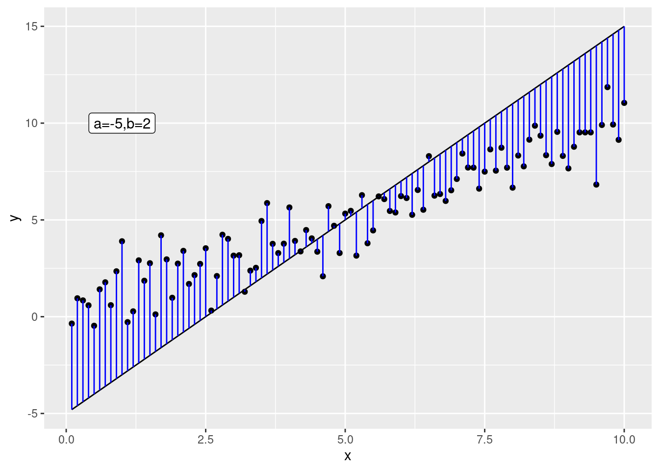
When fitting statistical models the aim is to “tweak” model settings until they can “mimic” the data optimally. In the case of linear regression we want to estimate the best line through a cloud of points:
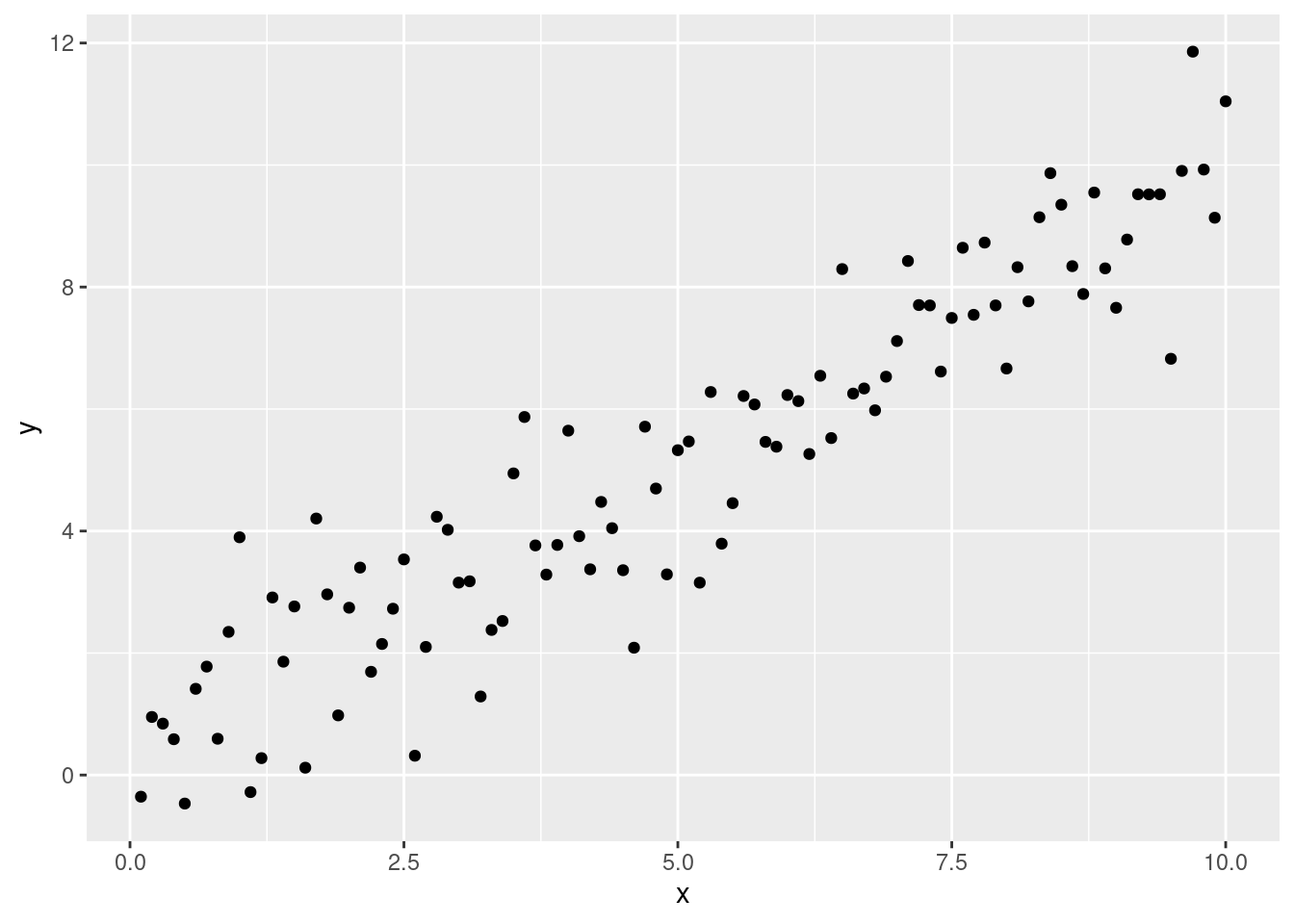
The best line is the one that minimizes the difference between the data and the (model) predictions. We want to choose parameters \(\beta_0\) and \(\beta_1\) such that this distance is minimized:
In addition to finding the optimal values of \(\beta_0\) and \(\beta_1\) we want to know if these values are significantly different from zero. In mathematical terms we want to draw inferences (hypothesis testing) of the form: \[H_0 : \qquad \beta = 0 \] vs. \[H_1 : \qquad \beta \neq 0 \]
Linear models in R
R provides a suite of tools for model building. Linear regression models are created using the lm function. Here we will use some simulated data to demonstrate model fitting.
dat <- tibble(x=1:100/10, y= x + rnorm(100,sd=1))
fit <- lm(y~x, data=dat)
fit
Call:
lm(formula = y ~ x, data = dat)

Coefficients:
(Intercept)            x
     0.2403       0.9620
where y~x is the formula based on which the parameters should be estimated, y is the dependent variable and x is explanatory variable and the ~ indicates that the variable x should be used to explain y.
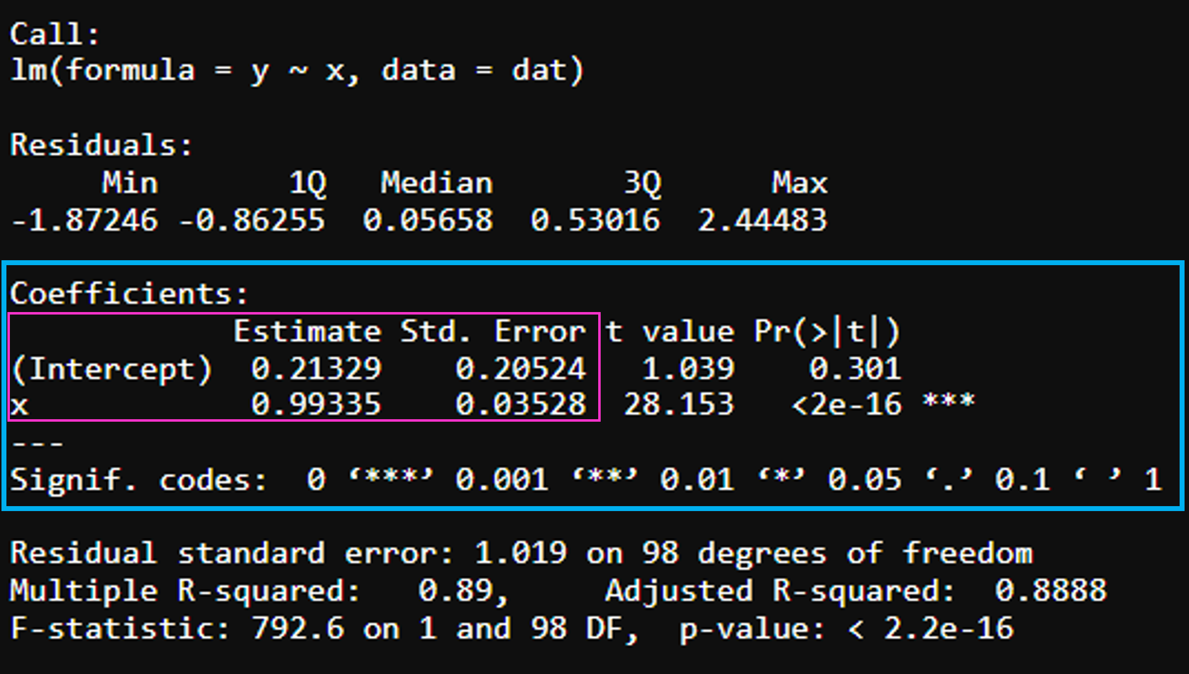
The lm function estimates the coefficients of the formula, and note that lm assumes that an intercept (\(\beta_0\)) is estimated as well as the slope (\(\beta_1\)). The summary function can then be used to view the model output and key statistics. The model coefficients are tabulated along with standard error estimates and p-values.
summary(fit)
Call:
lm(formula = y ~ x, data = dat)

Residuals:
     Min       1Q   Median       3Q      Max
-2.50856 -0.67352 -0.05555  0.61307  2.24964

Coefficients:
            Estimate Std. Error t value Pr(>|t|)
(Intercept)  0.24032    0.19794   1.214    0.228
x            0.96204    0.03403  28.271   <2e-16 ***
---
Signif. codes:  0 '***' 0.001 '**' 0.01 '*' 0.05 '.' 0.1 ' ' 1

Residual standard error: 0.9823 on 98 degrees of freedom
Multiple R-squared:  0.8908,    Adjusted R-squared:  0.8897
F-statistic: 799.2 on 1 and 98 DF,  p-value: < 2.2e-16
Demystifying R model output

Residuals
Residuals of the model showing median and interquartile range. Can use boxplots to check how symmetrical they are.
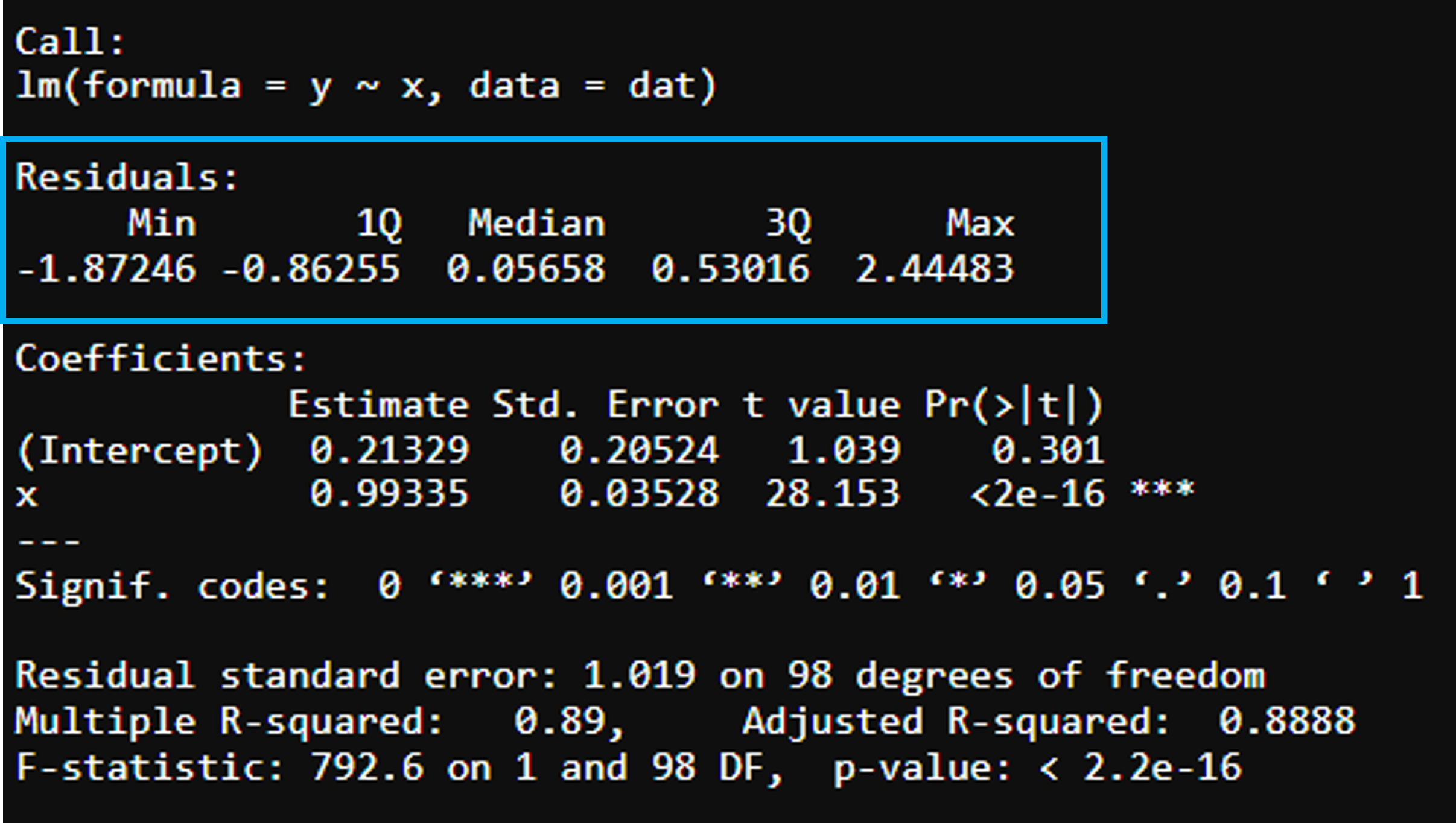
Model estimates
Intercept (\(\beta_0\)) - represents the mean value of the response variable when all of the predictor variables in the model are equal to zero
x (\(\beta_1\)) - is the expected difference in y for 1 unit increase in x
The coefficient’s standard error (St. Error) can be used to compute a confidence interval for the estimates.
Significance Level
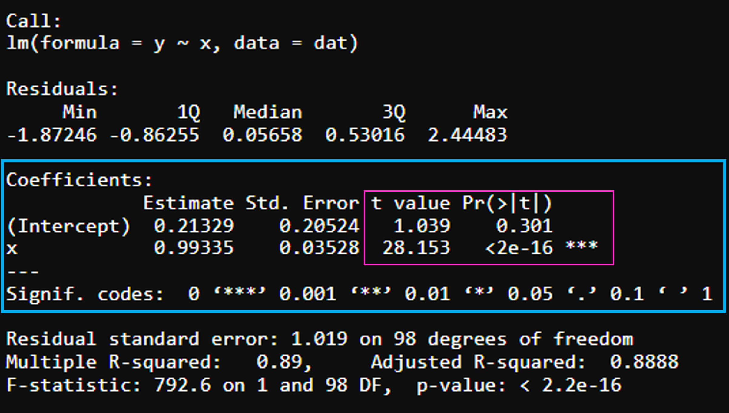
t-value – how many standard deviations the coefficient estimate is away from zero, want it to be far from 0!
Pr (>t) – probability of observing any value equal or higher than t, want small p, less than 5% is good.
The coefficient of the variable x is associated with a p-value < 0.05, therefore, we can say that x has a statistically significant effect on y
Goodness-of-fit
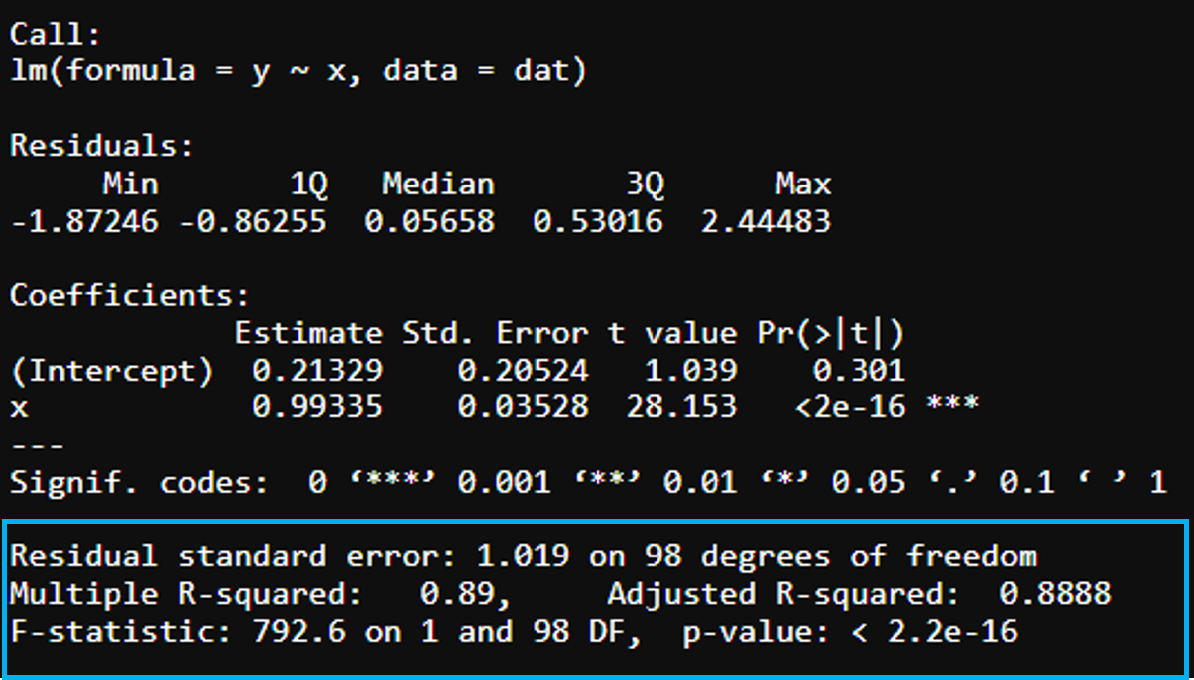
Residual standard error - measures how well the regression line fits the data. The smaller the better (100 data points, 2 parameter gives 98 degrees of freedom).
Multiple R-squared is the proportion of variance in y explained by the predictors Adjusted R-squared - Adjusts for number of variables considered (\(R^2\)) (will always increase with more variables that are included)
F-statistic - Indicator of whether there is a relationship between predictor and response variables, the further away from 1 the better
Compiling estimates in a tidy way
To extract these numbers explicitly as a data frame the broom package provides a nice function called tidy:
tidy(fit)# A tibble: 2 × 5
term estimate std.error statistic p.value
<chr> <dbl> <dbl> <dbl> <dbl>
1 (Intercept) 0.240 0.198 1.21 2.28e- 1
2 x 0.962 0.0340 28.3 6.42e-49and the confidence intervals can be calculated as:
tidy(fit,conf.int = TRUE)# A tibble: 2 × 7
term estimate std.error statistic p.value conf.low conf.high
<chr> <dbl> <dbl> <dbl> <dbl> <dbl> <dbl>
1 (Intercept) 0.240 0.198 1.21 2.28e- 1 -0.152 0.633
2 x 0.962 0.0340 28.3 6.42e-49 0.895 1.03 And to plot the prediction and residuals the modelr package has two functions, add_predictions and add_residuals:
aug.dat <-
dat %>%
add_predictions(fit) %>%
add_residuals(fit)
## plot predictions
aug.dat %>%
ggplot(aes(x,y)) + geom_point() + geom_line(aes(y=pred),col='blue')
## plot residuals
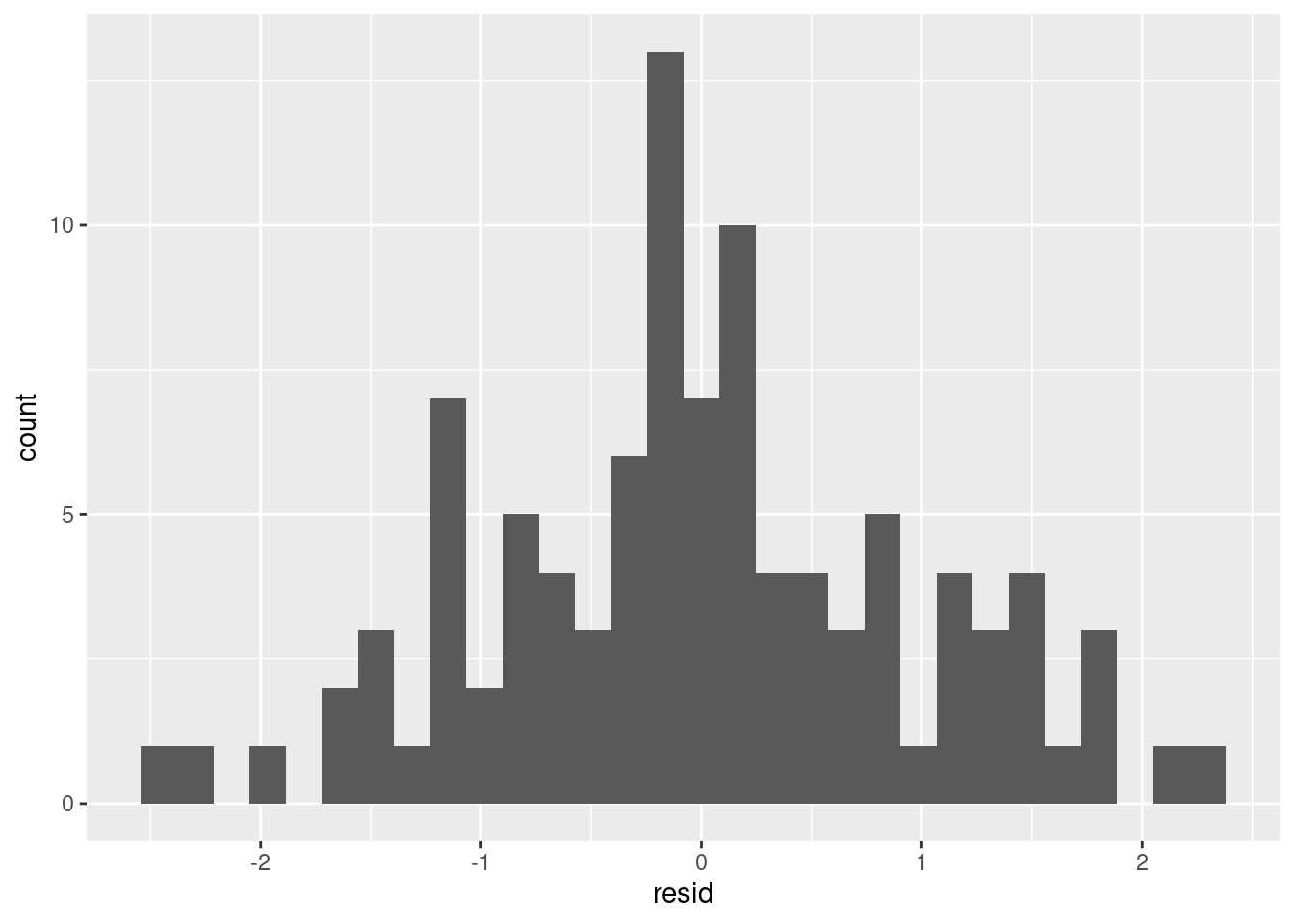
aug.dat %>%
ggplot(aes(resid)) + geom_histogram()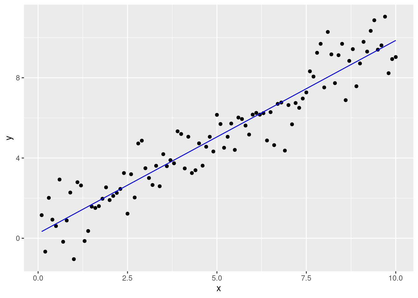
Model Diagnostics
For the model to be adequate, two main assumptions should hold:
- the error from the model should be normally distributed
- the homogeneity of variance (homoscedasticity) i.e the variance is equal and the error is constant along the values of the dependent variable
The diagnostic plots show residuals in four different ways:
- Residuals vs Fitted. Used to check the linear relationship assumptions. A horizontal line, without distinct patterns is an indication for a linear relationship (the red line should be more or less straight around 0).
plot(fit, 1)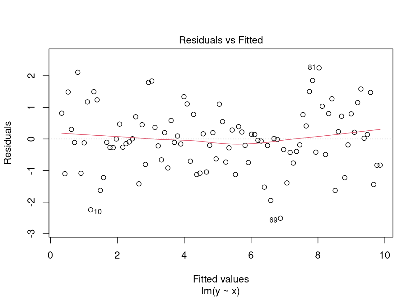
- Normal Q-Q plot. Used to examine whether the residuals are normally distributed. It’s good if residuals points follow the straight dashed line. Some deviations along the edges are acceptable.
plot(fit, 2)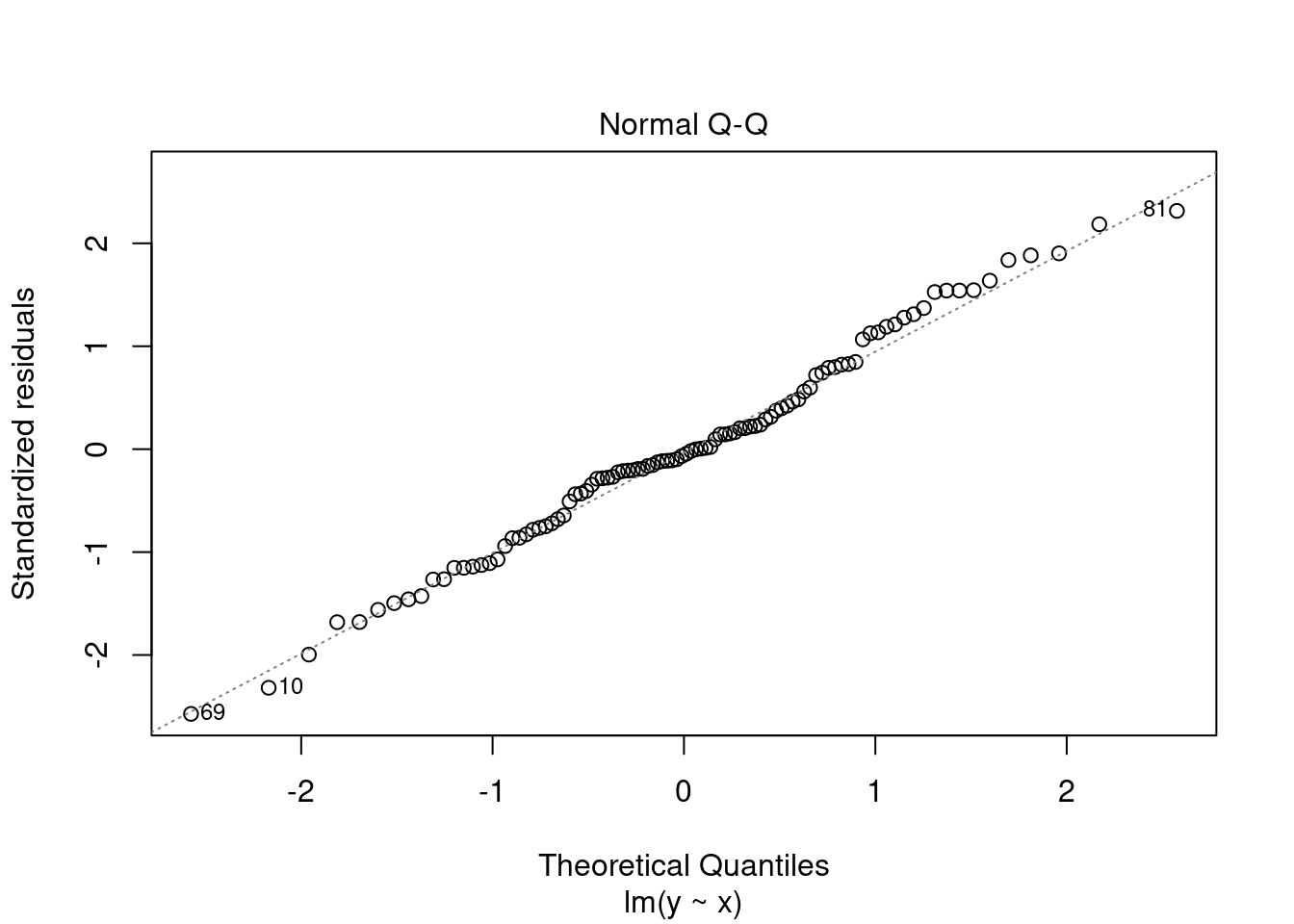
- Scale-Location (or Spread-Location). Used to check the homogeneity of variance of the residuals (homoscedasticity). Horizontal line with equally spread points is a good indication of homoscedasticity.
plot(fit, 3)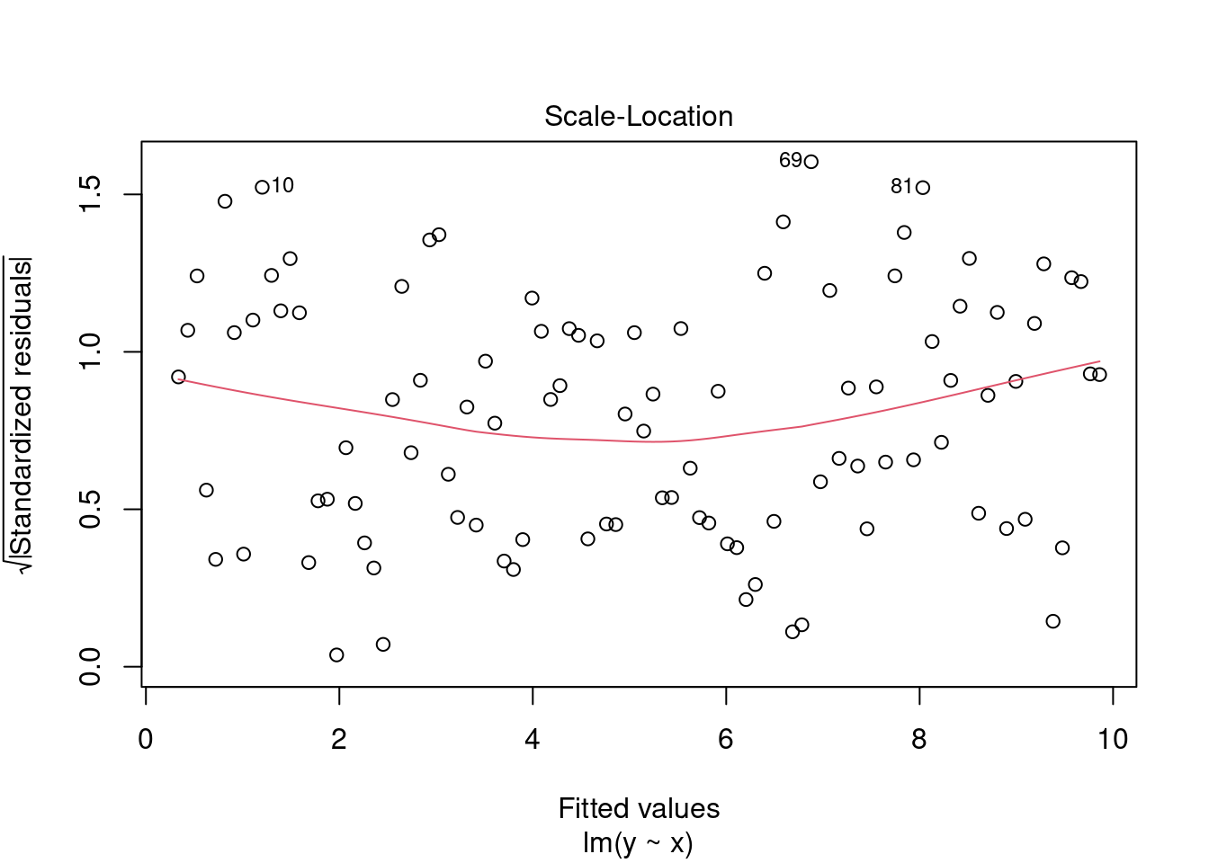
- Residuals vs Leverage. Used to identify influential cases, that is extreme values that might influence the regression results when included or excluded from the analysis. Will show outliers that may influence model fitting.
plot(fit, 4)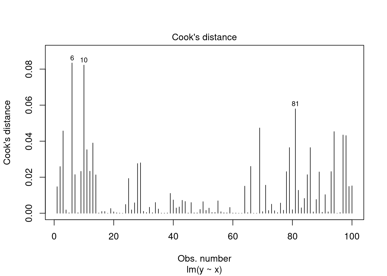
Fitting length and weight of cod
Now as a real example consider the length–weight relationship for cod.
d <- read_csv("https://heima.hafro.is/~einarhj/data/cod-survey-data.csv")

ggplot(d,aes(length,wgt,col=sex)) + geom_point()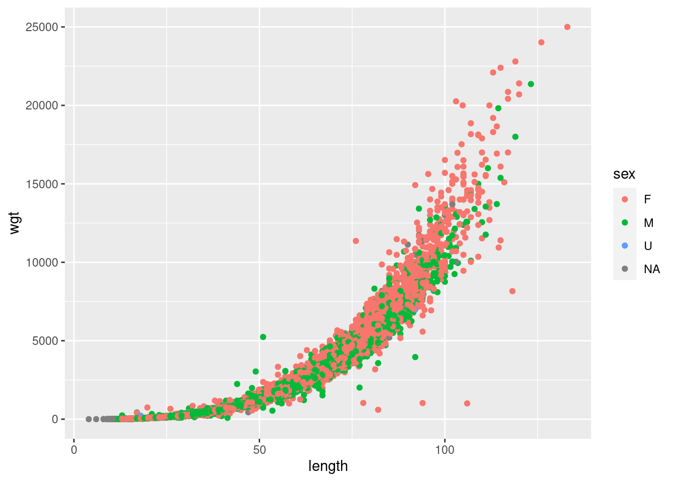
We see that the relationship between length and weight is probably not linear but as first approximation try that:
fit <- lm(wgt~length,data=d)
fit
Call:
lm(formula = wgt ~ length, data = d)

Coefficients:
(Intercept)       length
   -2414.08        91.57
hmm fish at 0 cm is -2.4 kg :) That is not really plausible. But look at the usual summaries:
summary(fit)
Call:
lm(formula = wgt ~ length, data = d)

Residuals:
    Min      1Q  Median      3Q     Max
-6286.0  -690.7  -283.3   549.7 15235.8

Coefficients:
              Estimate Std. Error t value Pr(>|t|)
(Intercept) -2414.0845    15.0576  -160.3   <2e-16 ***
length         91.5664     0.3178   288.2   <2e-16 ***
---
Signif. codes:  0 '***' 0.001 '**' 0.01 '*' 0.05 '.' 0.1 ' ' 1

Residual standard error: 1055 on 25234 degrees of freedom
Multiple R-squared:  0.7669,    Adjusted R-squared:  0.7669
F-statistic: 8.303e+04 on 1 and 25234 DF,  p-value: < 2.2e-16
Everything is highly significant, as you would expect with this wealth of data, but looking at the fit to the data and residual:
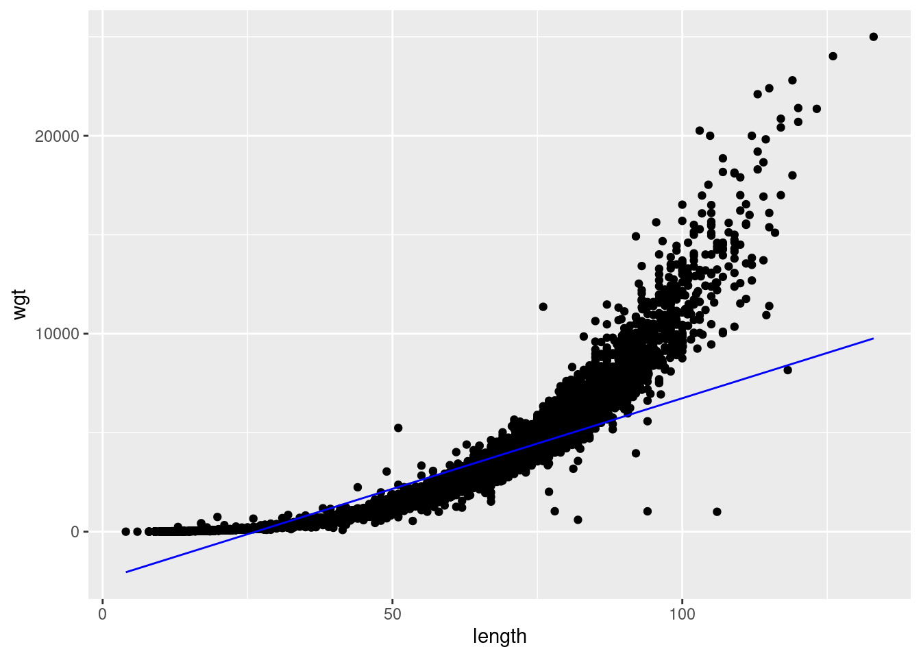
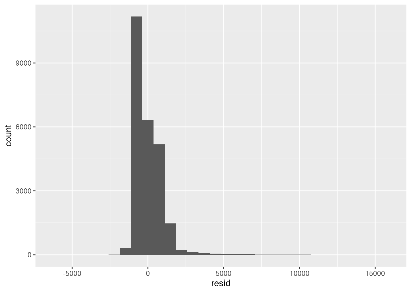
We see immediately that the model does not perform well on the tails and the residual error is heavily skewed. So let’s do something more realistic and log transform the data:
fit <- lm(log(wgt)~log(length),data=d)
fit
Call:
lm(formula = log(wgt) ~ log(length), data = d)

Coefficients:
(Intercept)  log(length)
     -5.077        3.127
This looks more sensible. Now lets plot the results:
aug.dat <-
  d %>%
  add_predictions(fit) %>%
  add_residuals(fit)
## plot predictions, note we need transform predictions back to non-log space
aug.dat %>%
  ggplot(aes(length,wgt)) + geom_point() + geom_line(aes(y=exp(pred)),col='blue')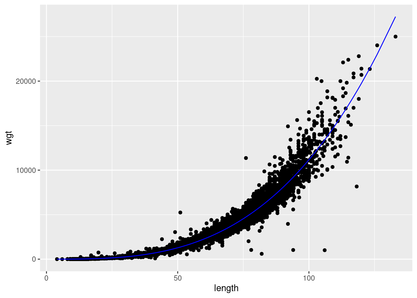
## plot residuals
aug.dat %>%
  ggplot(aes(resid)) + geom_histogram()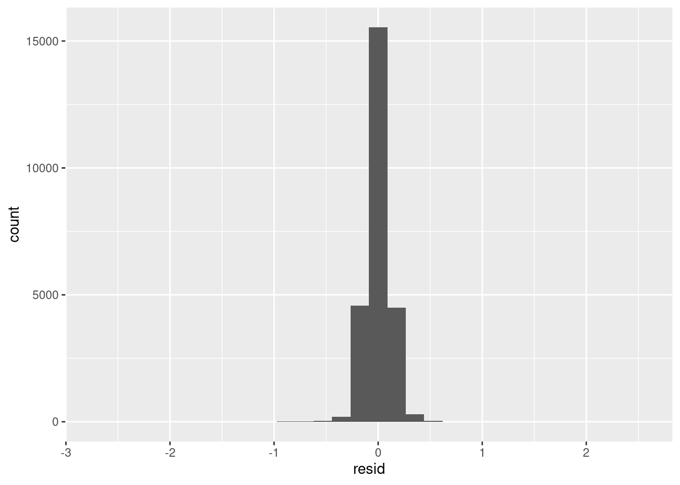
Test whether length-weight relationship differs by sex. Hint: We would have to add a new variable in the model using + variable name to be tested
fit2 <- lm(log(wgt) ~ log(length) + sex, data=d)
summary(fit2)
Generalized linear model
Model formulation and output
Generalized Linear models in R are formulated using the glm function
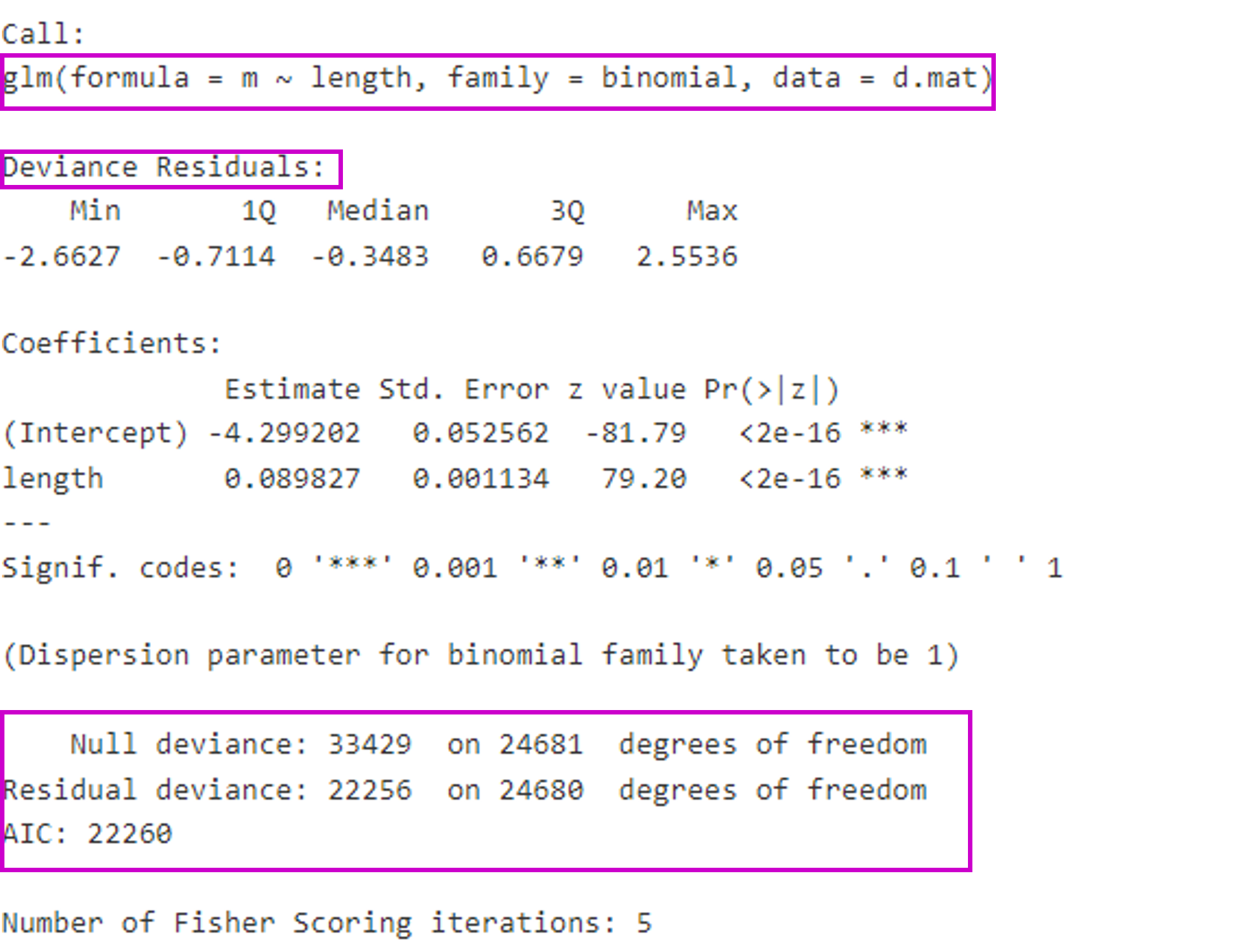
- The model output reports deviance instead of variance
Note there is no \(R^2\) reported but deviance explained can be obtained using
1 - residual deviance/null deviance)
Analysis of Variance (ANOVA)
ANOVA is essentially a test for the equality of means between two (or more) groups. ANOVA output is slightly different from linear model output because groups means are being tested. In R one uses aov function to test this class of hypotheses of whether groups means are different. The groups being tested have to be a categorical variable. In R one can use as.factor() or factor() to change a variable from being numeric to a category (factor).
One-way anova
As illustration of how one would perform an ANOVA in R consider the mean length caught by year:
ggplot(d,aes(year,length,group=round(year))) + geom_boxplot()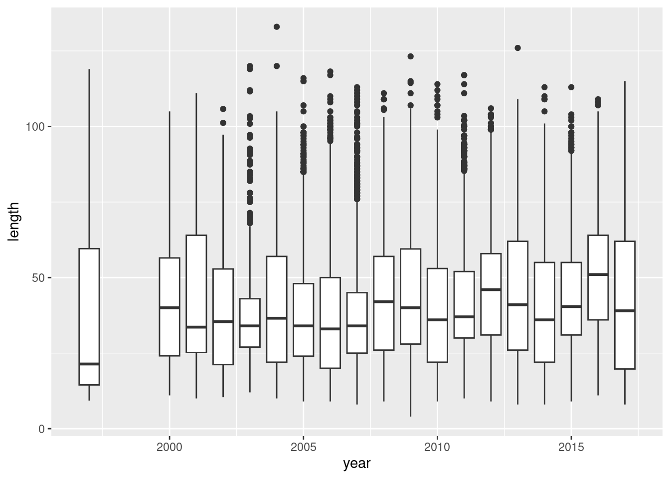
## note we need change the year to factor
fit <- aov(length~factor(year),data=d)
To get the results from the ANOVA one typically needs to use the summary function:
summary(fit) Df Sum Sq Mean Sq F value Pr(>F)
factor(year) 18 295620 16423 38.62 <2e-16 ***
Residuals 25217 10722244 425
---
Signif. codes: 0 '***' 0.001 '**' 0.01 '*' 0.05 '.' 0.1 ' ' 1where we see the mean length is significantly different by year. And as above we can use tidy
fit %>% tidy()# A tibble: 2 × 6
term df sumsq meansq statistic p.value
<chr> <dbl> <dbl> <dbl> <dbl> <dbl>
1 factor(year) 18 295620. 16423. 38.6 5.16e-134
2 Residuals 25217 10722244. 425. NA NA Now this is all well and good, but we now need to know which of these years are significantly different. This can be done using Tukey test, implemented using the lsmeans function:
fit %>% lsmeans(pairwise~year)$lsmeans
year lsmean SE df lower.CL upper.CL
1997 38.2 1.430 25217 35.4 41.0
2000 43.4 1.625 25217 40.2 46.6
2001 45.3 1.788 25217 41.8 48.8
2002 39.8 1.559 25217 36.7 42.8
2003 37.7 0.790 25217 36.2 39.3
2004 41.3 0.568 25217 40.1 42.4
2005 38.8 0.597 25217 37.6 40.0
2006 37.5 0.564 25217 36.4 38.6
2007 38.2 0.529 25217 37.1 39.2
2008 43.6 0.614 25217 42.4 44.8
2009 44.1 0.600 25217 42.9 45.3
2010 39.9 0.523 25217 38.9 40.9
2011 42.6 0.498 25217 41.6 43.6
2012 45.9 0.457 25217 45.0 46.8
2013 44.6 0.474 25217 43.7 45.6
2014 40.4 0.483 25217 39.5 41.4
2015 43.3 0.392 25217 42.5 44.1
2016 50.8 0.462 25217 49.9 51.7
2017 42.2 0.419 25217 41.3 43.0
Confidence level used: 0.95
$contrasts
contrast estimate SE df t.ratio p.value
year1997 - year2000 -5.1815 2.165 25217 -2.394 0.6403
year1997 - year2001 -7.1400 2.289 25217 -3.119 0.1604
year1997 - year2002 -1.5870 2.115 25217 -0.750 1.0000
year1997 - year2003 0.4373 1.634 25217 0.268 1.0000
year1997 - year2004 -3.0665 1.538 25217 -1.993 0.8905
year1997 - year2005 -0.6273 1.549 25217 -0.405 1.0000
year1997 - year2006 0.7222 1.537 25217 0.470 1.0000
year1997 - year2007 0.0205 1.525 25217 0.013 1.0000
year1997 - year2008 -5.3735 1.556 25217 -3.454 0.0612
year1997 - year2009 -5.8945 1.550 25217 -3.802 0.0187
year1997 - year2010 -1.7129 1.522 25217 -1.125 0.9998
year1997 - year2011 -4.4357 1.514 25217 -2.930 0.2537
year1997 - year2012 -7.6884 1.501 25217 -5.122 <.0001
year1997 - year2013 -6.4512 1.506 25217 -4.283 0.0028
year1997 - year2014 -2.2517 1.509 25217 -1.492 0.9937
year1997 - year2015 -5.1015 1.482 25217 -3.441 0.0637
year1997 - year2016 -12.6096 1.503 25217 -8.392 <.0001
year1997 - year2017 -3.9715 1.490 25217 -2.666 0.4296
year2000 - year2001 -1.9585 2.416 25217 -0.811 1.0000
year2000 - year2002 3.5945 2.252 25217 1.596 0.9865
year2000 - year2003 5.6188 1.807 25217 3.109 0.1644
year2000 - year2004 2.1150 1.721 25217 1.229 0.9995
year2000 - year2005 4.5542 1.731 25217 2.630 0.4564
year2000 - year2006 5.9037 1.720 25217 3.432 0.0655
year2000 - year2007 5.2020 1.709 25217 3.044 0.1940
year2000 - year2008 -0.1920 1.737 25217 -0.111 1.0000
year2000 - year2009 -0.7130 1.732 25217 -0.412 1.0000
year2000 - year2010 3.4686 1.707 25217 2.032 0.8731
year2000 - year2011 0.7458 1.700 25217 0.439 1.0000
year2000 - year2012 -2.5069 1.688 25217 -1.485 0.9940
year2000 - year2013 -1.2697 1.693 25217 -0.750 1.0000
year2000 - year2014 2.9298 1.695 25217 1.728 0.9693
year2000 - year2015 0.0800 1.672 25217 0.048 1.0000
year2000 - year2016 -7.4281 1.690 25217 -4.396 0.0017
year2000 - year2017 1.2100 1.678 25217 0.721 1.0000
year2001 - year2002 5.5530 2.372 25217 2.341 0.6802
year2001 - year2003 7.5773 1.955 25217 3.876 0.0142
year2001 - year2004 4.0734 1.876 25217 2.171 0.7966
year2001 - year2005 6.5126 1.885 25217 3.455 0.0610
year2001 - year2006 7.8621 1.875 25217 4.194 0.0040
year2001 - year2007 7.1605 1.865 25217 3.840 0.0162
year2001 - year2008 1.7665 1.890 25217 0.934 1.0000
year2001 - year2009 1.2455 1.886 25217 0.660 1.0000
year2001 - year2010 5.4271 1.863 25217 2.913 0.2631
year2001 - year2011 2.7042 1.856 25217 1.457 0.9952
year2001 - year2012 -0.5484 1.846 25217 -0.297 1.0000
year2001 - year2013 0.6888 1.850 25217 0.372 1.0000
year2001 - year2014 4.8883 1.852 25217 2.639 0.4496
year2001 - year2015 2.0385 1.830 25217 1.114 0.9999
year2001 - year2016 -5.4696 1.847 25217 -2.962 0.2358
year2001 - year2017 3.1685 1.836 25217 1.725 0.9698
year2002 - year2003 2.0243 1.748 25217 1.158 0.9998
year2002 - year2004 -1.4795 1.659 25217 -0.892 1.0000
year2002 - year2005 0.9597 1.669 25217 0.575 1.0000
year2002 - year2006 2.3091 1.658 25217 1.393 0.9972
year2002 - year2007 1.6075 1.646 25217 0.976 1.0000
year2002 - year2008 -3.7865 1.675 25217 -2.260 0.7382
year2002 - year2009 -4.3075 1.670 25217 -2.579 0.4958
year2002 - year2010 -0.1259 1.644 25217 -0.077 1.0000
year2002 - year2011 -2.8487 1.636 25217 -1.741 0.9670
year2002 - year2012 -6.1014 1.624 25217 -3.756 0.0221
year2002 - year2013 -4.8642 1.629 25217 -2.985 0.2231
year2002 - year2014 -0.6647 1.632 25217 -0.407 1.0000
year2002 - year2015 -3.5145 1.607 25217 -2.187 0.7871
year2002 - year2016 -11.0226 1.626 25217 -6.780 <.0001
year2002 - year2017 -2.3845 1.614 25217 -1.477 0.9944
year2003 - year2004 -3.5038 0.973 25217 -3.601 0.0378
year2003 - year2005 -1.0646 0.990 25217 -1.075 0.9999
year2003 - year2006 0.2849 0.971 25217 0.293 1.0000
year2003 - year2007 -0.4168 0.951 25217 -0.438 1.0000
year2003 - year2008 -5.8108 1.000 25217 -5.808 <.0001
year2003 - year2009 -6.3317 0.992 25217 -6.383 <.0001
year2003 - year2010 -2.1501 0.947 25217 -2.270 0.7317
year2003 - year2011 -4.8730 0.934 25217 -5.216 <.0001
year2003 - year2012 -8.1257 0.913 25217 -8.900 <.0001
year2003 - year2013 -6.8885 0.922 25217 -7.474 <.0001
year2003 - year2014 -2.6890 0.926 25217 -2.903 0.2690
year2003 - year2015 -5.5388 0.882 25217 -6.280 <.0001
year2003 - year2016 -13.0469 0.915 25217 -14.252 <.0001
year2003 - year2017 -4.4088 0.894 25217 -4.931 0.0001
year2004 - year2005 2.4392 0.824 25217 2.961 0.2365
year2004 - year2006 3.7887 0.800 25217 4.735 0.0003
year2004 - year2007 3.0871 0.776 25217 3.977 0.0096
year2004 - year2008 -2.3070 0.836 25217 -2.760 0.3616
year2004 - year2009 -2.8279 0.826 25217 -3.425 0.0670
year2004 - year2010 1.3537 0.771 25217 1.755 0.9644
year2004 - year2011 -1.3692 0.755 25217 -1.813 0.9515
year2004 - year2012 -4.6218 0.729 25217 -6.340 <.0001
year2004 - year2013 -3.3847 0.740 25217 -4.576 0.0007
year2004 - year2014 0.8149 0.745 25217 1.093 0.9999
year2004 - year2015 -2.0350 0.690 25217 -2.951 0.2418
year2004 - year2016 -9.5431 0.732 25217 -13.037 <.0001
year2004 - year2017 -0.9050 0.705 25217 -1.283 0.9990
year2005 - year2006 1.3495 0.821 25217 1.643 0.9817
year2005 - year2007 0.6479 0.798 25217 0.812 1.0000
year2005 - year2008 -4.7462 0.856 25217 -5.542 <.0001
year2005 - year2009 -5.2671 0.846 25217 -6.223 <.0001
year2005 - year2010 -1.0855 0.794 25217 -1.368 0.9978
year2005 - year2011 -3.8084 0.778 25217 -4.896 0.0002
year2005 - year2012 -7.0610 0.752 25217 -9.386 <.0001
year2005 - year2013 -5.8239 0.763 25217 -7.636 <.0001
year2005 - year2014 -1.6243 0.768 25217 -2.115 0.8302
year2005 - year2015 -4.4742 0.714 25217 -6.264 <.0001
year2005 - year2016 -11.9823 0.755 25217 -15.866 <.0001
year2005 - year2017 -3.3442 0.729 25217 -4.585 0.0007
year2006 - year2007 -0.7016 0.774 25217 -0.907 1.0000
year2006 - year2008 -6.0957 0.833 25217 -7.314 <.0001
year2006 - year2009 -6.6166 0.823 25217 -8.037 <.0001
year2006 - year2010 -2.4350 0.769 25217 -3.167 0.1412
year2006 - year2011 -5.1579 0.753 25217 -6.854 <.0001
year2006 - year2012 -8.4105 0.726 25217 -11.583 <.0001
year2006 - year2013 -7.1733 0.737 25217 -9.735 <.0001
year2006 - year2014 -2.9738 0.743 25217 -4.005 0.0086
year2006 - year2015 -5.8237 0.687 25217 -8.481 <.0001
year2006 - year2016 -13.3317 0.729 25217 -18.283 <.0001
year2006 - year2017 -4.6937 0.702 25217 -6.683 <.0001
year2007 - year2008 -5.3940 0.810 25217 -6.655 <.0001
year2007 - year2009 -5.9150 0.800 25217 -7.394 <.0001
year2007 - year2010 -1.7334 0.744 25217 -2.330 0.6882
year2007 - year2011 -4.4563 0.727 25217 -6.129 <.0001
year2007 - year2012 -7.7089 0.700 25217 -11.018 <.0001
year2007 - year2013 -6.4717 0.711 25217 -9.105 <.0001
year2007 - year2014 -2.2722 0.717 25217 -3.170 0.1400
year2007 - year2015 -5.1220 0.659 25217 -7.777 <.0001
year2007 - year2016 -12.6301 0.703 25217 -17.971 <.0001
year2007 - year2017 -3.9920 0.675 25217 -5.915 <.0001
year2008 - year2009 -0.5210 0.858 25217 -0.607 1.0000
year2008 - year2010 3.6606 0.806 25217 4.541 0.0009
year2008 - year2011 0.9378 0.791 25217 1.186 0.9997
year2008 - year2012 -2.3149 0.765 25217 -3.024 0.2033
year2008 - year2013 -1.0777 0.776 25217 -1.389 0.9973
year2008 - year2014 3.1218 0.781 25217 3.997 0.0089
year2008 - year2015 0.2720 0.728 25217 0.374 1.0000
year2008 - year2016 -7.2361 0.768 25217 -9.418 <.0001
year2008 - year2017 1.4020 0.743 25217 1.887 0.9304
year2009 - year2010 4.1816 0.795 25217 5.257 <.0001
year2009 - year2011 1.4587 0.780 25217 1.871 0.9356
year2009 - year2012 -1.7939 0.754 25217 -2.378 0.6522
year2009 - year2013 -0.5567 0.765 25217 -0.728 1.0000
year2009 - year2014 3.6428 0.770 25217 4.730 0.0004
year2009 - year2015 0.7930 0.716 25217 1.107 0.9999
year2009 - year2016 -6.7151 0.757 25217 -8.868 <.0001
year2009 - year2017 1.9229 0.731 25217 2.629 0.4573
year2010 - year2011 -2.7229 0.722 25217 -3.771 0.0209
year2010 - year2012 -5.9755 0.695 25217 -8.604 <.0001
year2010 - year2013 -4.7383 0.706 25217 -6.714 <.0001
year2010 - year2014 -0.5388 0.712 25217 -0.757 1.0000
year2010 - year2015 -3.3886 0.653 25217 -5.189 <.0001
year2010 - year2016 -10.8967 0.698 25217 -15.619 <.0001
year2010 - year2017 -2.2586 0.670 25217 -3.373 0.0784
year2011 - year2012 -3.2526 0.676 25217 -4.808 0.0002
year2011 - year2013 -2.0155 0.688 25217 -2.929 0.2538
year2011 - year2014 2.1841 0.694 25217 3.147 0.1491
year2011 - year2015 -0.6658 0.634 25217 -1.050 0.9999
year2011 - year2016 -8.1739 0.680 25217 -12.025 <.0001
year2011 - year2017 0.4642 0.651 25217 0.713 1.0000
year2012 - year2013 1.2372 0.659 25217 1.878 0.9335
year2012 - year2014 5.4367 0.665 25217 8.172 <.0001
year2012 - year2015 2.5869 0.602 25217 4.295 0.0026
year2012 - year2016 -4.9212 0.650 25217 -7.567 <.0001
year2012 - year2017 3.7169 0.620 25217 5.995 <.0001
year2013 - year2014 4.1995 0.677 25217 6.203 <.0001
year2013 - year2015 1.3497 0.615 25217 2.194 0.7824
year2013 - year2016 -6.1584 0.662 25217 -9.299 <.0001
year2013 - year2017 2.4797 0.633 25217 3.920 0.0120
year2014 - year2015 -2.8498 0.622 25217 -4.582 0.0007
year2014 - year2016 -10.3579 0.669 25217 -15.492 <.0001
year2014 - year2017 -1.7198 0.639 25217 -2.691 0.4112
year2015 - year2016 -7.5081 0.606 25217 -12.392 <.0001
year2015 - year2017 1.1300 0.573 25217 1.971 0.9000
year2016 - year2017 8.6381 0.624 25217 13.852 <.0001
P value adjustment: tukey method for comparing a family of 19 estimates But getting the results to a data.frame is bit more involved:
ls.fit <- fit %>% lsmeans(pairwise~year)
ls.cont <- ls.fit$contrasts %>% summary() %>% as_data_frame()
ls.cont
# A tibble: 171 × 6
contrast estimate SE df t.ratio p.value
<chr> <dbl> <dbl> <dbl> <dbl> <dbl>
1 year1997 - year2000 -5.18 2.16 25217 -2.39 0.640
2 year1997 - year2001 -7.14 2.29 25217 -3.12 0.160
3 year1997 - year2002 -1.59 2.12 25217 -0.750 1.00
4 year1997 - year2003 0.437 1.63 25217 0.268 1
5 year1997 - year2004 -3.07 1.54 25217 -1.99 0.891
6 year1997 - year2005 -0.627 1.55 25217 -0.405 1.00
7 year1997 - year2006 0.722 1.54 25217 0.470 1.00
8 year1997 - year2007 0.0205 1.52 25217 0.0135 1
9 year1997 - year2008 -5.37 1.56 25217 -3.45 0.0612
10 year1997 - year2009 -5.89 1.55 25217 -3.80 0.0187
# ℹ 161 more rowsAnd to find the years:
ls.cont %>% filter(p.value < 0.05)# A tibble: 73 × 6
contrast estimate SE df t.ratio p.value
<chr> <dbl> <dbl> <dbl> <dbl> <dbl>
1 year1997 - year2009 -5.89 1.55 25217 -3.80 1.87e- 2
2 year1997 - year2012 -7.69 1.50 25217 -5.12 5.00e- 5
3 year1997 - year2013 -6.45 1.51 25217 -4.28 2.75e- 3
4 year1997 - year2016 -12.6 1.50 25217 -8.39 2.03e-13
5 year2000 - year2016 -7.43 1.69 25217 -4.40 1.68e- 3
6 year2001 - year2003 7.58 1.95 25217 3.88 1.42e- 2
7 year2001 - year2006 7.86 1.87 25217 4.19 4.02e- 3
8 year2001 - year2007 7.16 1.86 25217 3.84 1.62e- 2
9 year2002 - year2012 -6.10 1.62 25217 -3.76 2.21e- 2
10 year2002 - year2016 -11.0 1.63 25217 -6.78 2.06e- 9
# ℹ 63 more rowsTest if weight is significantly different by year
fit2 <- aov(wgt~factor(year),data=d)
summary(fit2)