Introduction
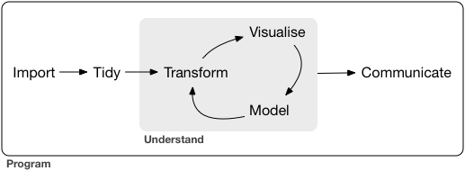
Typical science project
- Import
- Import data stored in a file, database, or web API, and load it into R
- Tidy
- Each column is a variable, and each row is an observation
Tidy datasets are all alike but every messy dataset is messy in its own way.
- Hadley Wickham- Transform
- Narrowing in on observations of interest
- Creating new variables that are functions of existing variables
- Calculating a set of summary statistics (like counts or means)
- …
- Visualize
- May show unexpected things
- May raise new questions about the data
- A powerful communication platform
- …
- Model
- Once questions are made sufficiently precise, one can create a hypothesis and use a model test it
- Model cannot question its own assumptions, hence Bayesian approach may be more Kosher
- Communicate
- Presentation and documentation
Our aim
Our aim in this short course is to:
- Get you up and running with importing, visualization, transformation and summarisation of fisheries data.
- Introduce you to programming, including modelling in R
- Get you a head start with analyzing your own data in R.
- Introduce you to reproducible analysis and document writing.
- Touch upon the fundamentals of fisheries assessment.
We are going to use a set of tools that fall under the tidyverse umbrella. These are basic set of generic tools that are integrated to work seamlessly with one another.
We believe that the tools introduced will get your quickly up and running with your own data, solving >50% of the most common tasks. Going through the R for Data Science by Grolemund and Hadley (which serves as our basic template for some of course structure) will pick up additional 30+%.
R
What is R?
- R is command line driven programming language
- its biggest appeal is one can reuse commands
- its biggest hurdle in widespread use
In MS Excel you see the data but not the code
In        R you see the code but not the data

When explaining your method in     R - you just    share the code
When explaining your method in Excel - you need to share the data- R is open-source:
- Other statistical software packages can be extremely expensive
- Large user base with almost all statistical methods implemented
Why R?
R has become the lingua franca of statistical analysis and data wrangling in fisheries science (at least in Europe).
- Its free! If you are a teacher, a student or a user, the benefits are obvious
- It runs on a variety of platforms including Windows, Unix and MacOS
- It provides an unparalleled platform for programming new statistical methods in an easy and straightforward manner
- It offers powerful tools for data exploration and presentation
- It has ample resources on the web
But there are other open source free software out there (e.g. python) that can also achive similar tasks.
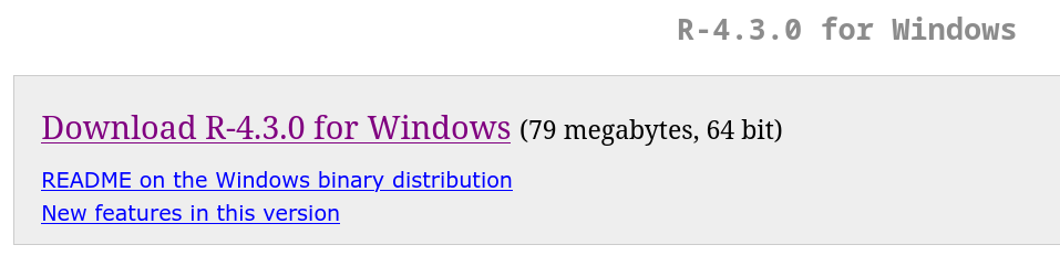
Installing R
Latest version of R: see The Comprehensive R Archive Network. Follow the instructions to complete the installation process:
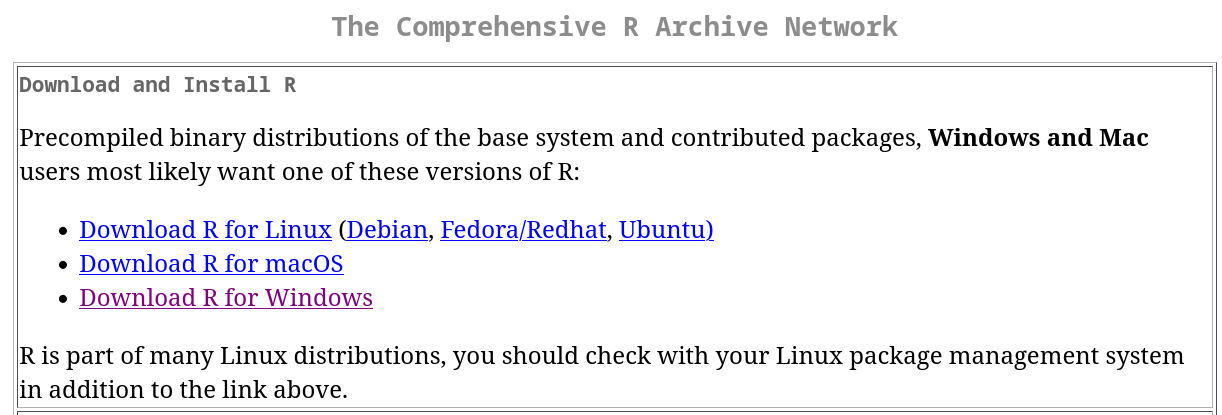
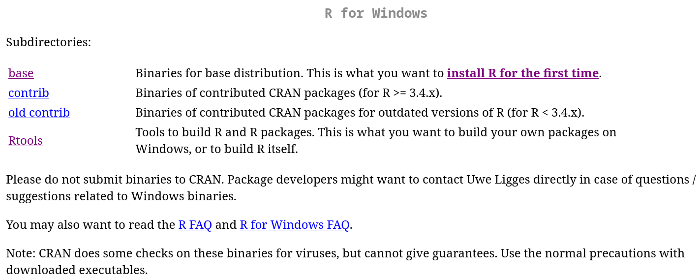
If your platform is Windows, it is recommended that you install Rtools
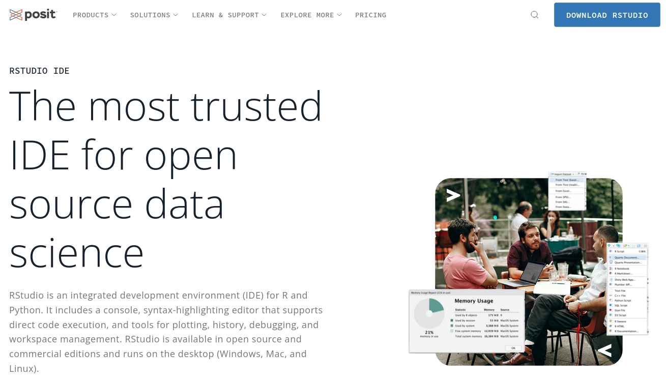
RStudio
What is RStudio?
- RStudio is an integrated development environment (IDE)
- It is open-source and free.
- Built to help you write R code, run R code, and analyze data with R
- Text editor, project handling, markdown support, keyboard shortcuts, debugging tools, version control, …
- Within RStudio one can achieve almost all that is needed to complete a typical science project, be it:
- A technical report
- A scientific manuscript
- Web pages (including blogs)
- …
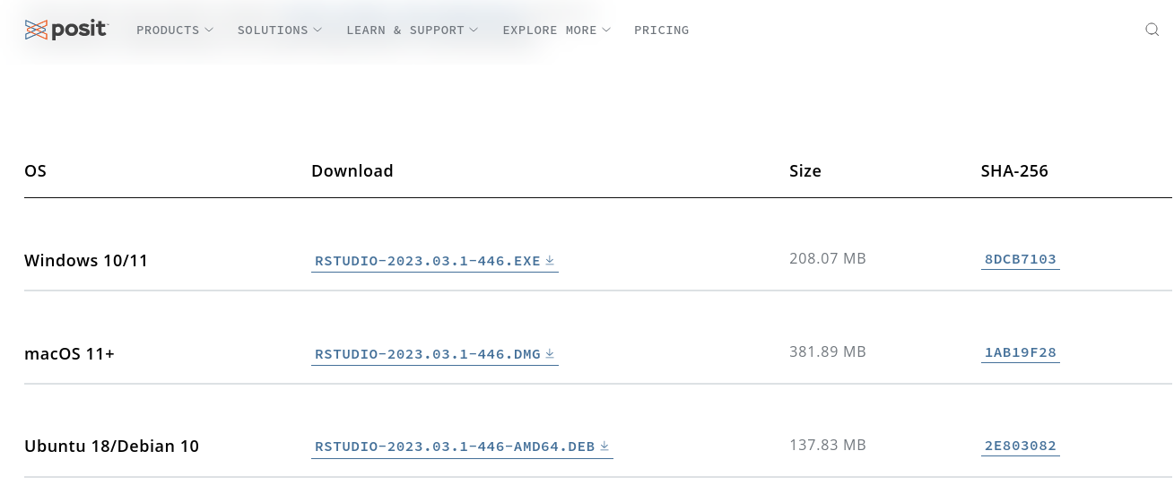
Intalling RStudio
Latest version of RStudio Desktop can be obtained from this link
Running RStudio
A typical RStudio window may look something like this:
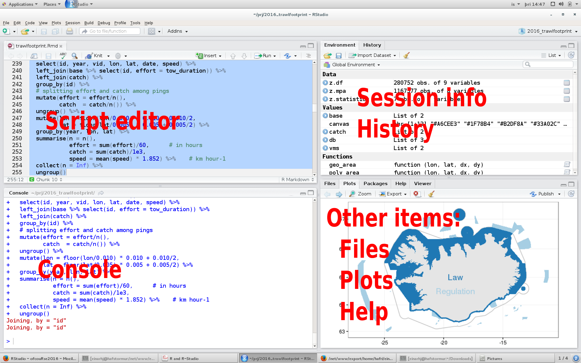
- Script editor: This is where you write the code for your analysis. These could include:
- R script - An R script is basically a series of stored R commands that can be run in the console - To generate a new script do: New file -> R Script (ctrl-shift-N)
- Rmarkdown document: A document with (or without) R-code.
- Console: This is where R prints the output of your code when it’s run. You can also write code directly in the console after the
>symbol, but that code is not preserved. - Environment/History: Have at minimum the following tabs:
- Environment: Displays all your obtjects (data) and user-defined functions in your current session. One can click on the objects to get a detailed view.
- History: Contains a list of previous commands entered into the console
- Additional tabs may include:
- Connection: Any database connections
- Build: If your project is webpage/blog project
- Git: If your project has version control
- Tutorial: Some nice basic tutorials on R
- Files/Packages/Help/Viewer:
- Files - The list of all files contained in your current working directory. You can also:
- Navigate to different folders on your computer.
- Create new blank files or folders (directories)
- Delete files or folders
- Rename files or folders
- … More
- Plots - Graphical output from R. The user can export the figures to file (as jpeg, png or pdf) or to clipboard
- Packages - The list of packages (groups of functions) currently installed on your computer. You can install new packages or update existing packages from this tab by clicking
InstallorUpdate. - Help - Search R documentation to get information what each function does and how. Using the help should be your first stop when trying to figure out how to use a particular function. The lingo may be intitially unfamiliar but with frequent use it becomes more bearable.
- Viewer: For interactive graphics
- Files - The list of all files contained in your current working directory. You can also:
RStudio project
- RStudio allows us to make things a little bit easier by isolating various tasks within specific projects (read: directory/folder on your computer).
- Projects save the state between sessions. This includes:
- Working directories
- Open files/scripts
- Workspaces (.RData file - do not save this)
- One can have multiple RStudio projects open at any one time
We strongly urge you to get into the habit of splitting your various tasks into specific RStudio projects.
RStudio project and our first code
- Open RStudio and create a new project: File -> New project … -> New directory –> Empty project –> …
- Create a new R script: File -> New file -> R Script
- Copy this to the script:
1 + 1- Pass the script to the console by putting the cursor on the code line and press ctrl-enter.
- Save the script, e.g. “doodle.R”: File -> Save
Global options
When you install RStudio it comes with a set of default options. You can change the defaults by doing: Tools -> Global Options…
We strongly urge you to changes at minimum two of the options:
- General - Workspace:
- No tickmark before “Restore .RData into workspace at startup”
- Select “Never” after “Save workspace to .RData on exit”
- R Markdown
- No tickmark before “Show output inline for all R Markdown documents
Packages
What are packages?
- Packages are a collection of functions and data with documentations.
- Numerous basic packages come with R but the strength of the R-environment comes from the huge amount of packages that are provided by third sources.
Installing packages
We may as well install/update the core packages that we will use in the coming days. Lets try to run the following (We would be surprised if this works for everybody in the first go):
install.packages("tidyverse")This will install among other things the core tidyverse packages:
- ggplot2, for data visualization.
- dplyr, for data manipulation.
- tidyr, for data tidying.
- readr, for data import.
- purrr, for functional programming.
- tibble, for “tibbles”, a modern re-imagining of data frames.
- stringr, for strings
- forcats, for factors
- lubridate, for date/times
library(tidyverse) will load these core tidyverse packages.
Additional packages will be install as we progress through the course.
Our first real project
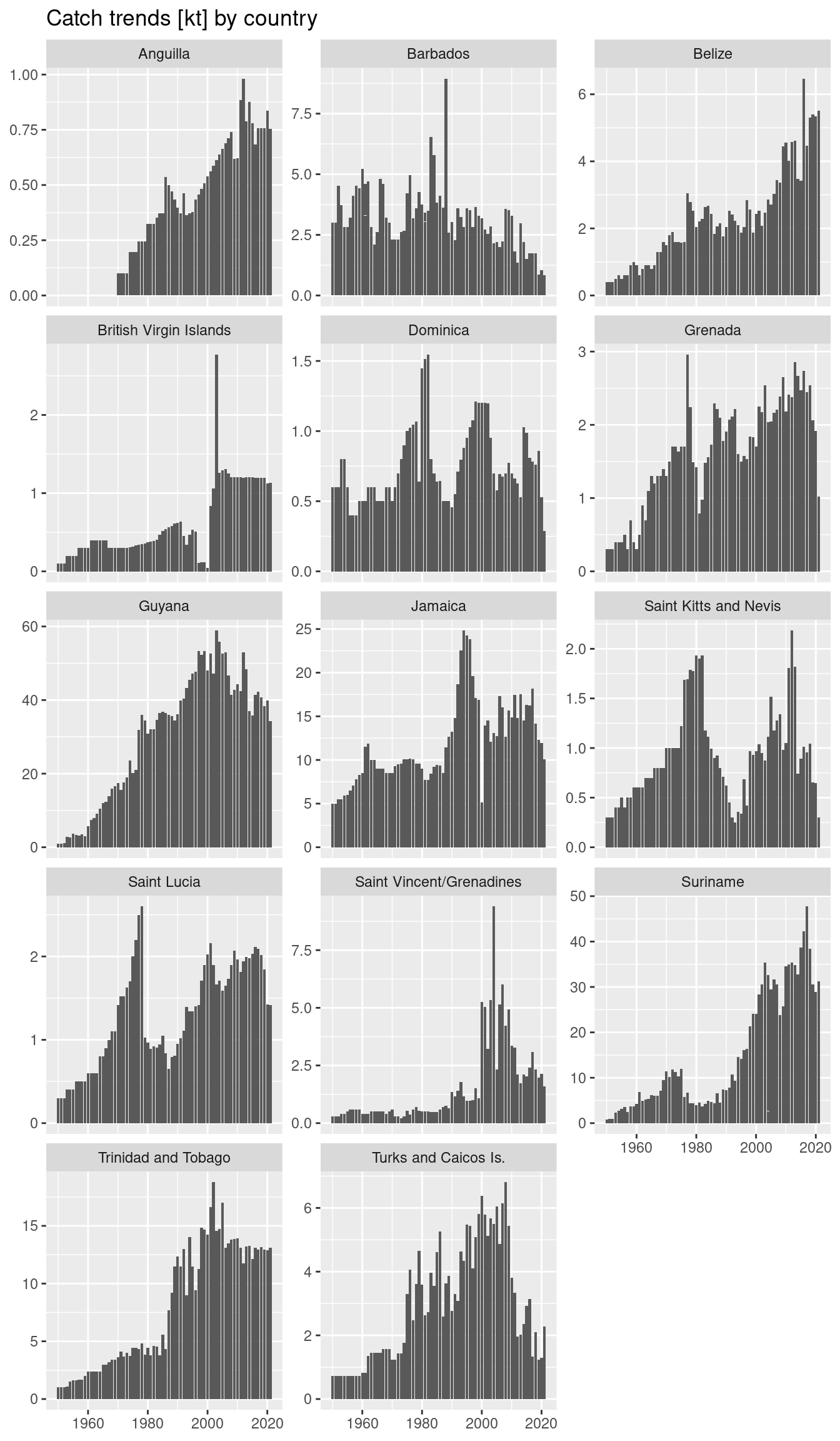
Exercise: Catch by country
- Open R-studio and create a new project: File -> New project … -> New directory –> Empty project –> …
- Create a new R script: File -> New file -> R Script
- Copy this to the script (if you are new to R this code is latin to you - do not worry, we will cover the details of it at a later stage).
library(tidyverse)
fao <- read_csv("https://heima.hafro.is/~einarhj/data/fao-capture-statistics_area31.csv")
my_country <- "Barbados"      # replace with your country name (see option list below)
fao |>
  filter(country %in% my_country) |>
  ggplot(aes(year, catch)) +
  geom_col()
The country names options are:
Anguilla
Belize
Barbados
British Virgin Islands
Dominica
Grenada
Guyana
Jamaica
Saint Kitts and Nevis
Saint Lucia
Saint Vincent/Grenadines"
Suriname
Trinidad and Tobago
Turks and Caicos Is.- Save the script, e.g. “fao.R”: File -> Save
- Pass the script to the Console by putting the cursor on the code line in the first line and press ctrl-enter is succession (or press the green “Run”-button).
Result (click me):
If you are interested to know more about the data and how it was obtained check the Data section.
The course material
The course material is open source, meaning that the source code is made freely available and may be redistributed and modified.
- The source code for the course material is located at: https://github.com/fishvice/crfmr
- The course product is rendered at: https://heima.hafro.is/~einarhj/crfmr
The material is largely based on the works of R for Data Science (2e)
Readings
Three books that we recommend you start off with:
- R for Data Science (2e)
- ggplot2: Elegant Graphics for Data Analysis (3e)
- R Markdown: The Definitive Guide
Disclaimer: Although Rmarkdown will remain available, new features will not be add because the author realized the base of the platform has limitation. This markdown system is called quarto. Since this platform is only 4 months old it was not presented in this course.