Exploratory data analysis

Preamble

Exploratory data analysis fall under the umbrella of tidying, transforming, visualization and possibly modelling. EDA involves among other things:

• Familiarization of the data
• Detecting patterns and trends
• You may discover some new patterns in your own data
• A precursor to hypothesis testing

In this section we are going to use the Icelandic trawl groundfish survey as a case example in EDA, covering some transformations and more visualization techniques along the way.

The survey falls under the realm of standardized scientific survey where the idea is that the gear design and the effort is kept as constant as possible over the years with the output then being survey indicies to be used as input into stock assessment.

The concept with the code below is to present the idea that one can extract information, knowledge and pattern in the data without much external knowledge. That said knowing your data, sampling design, including potential pitfalls. shortcomings, etc. is vital.

Ad hoc EDA

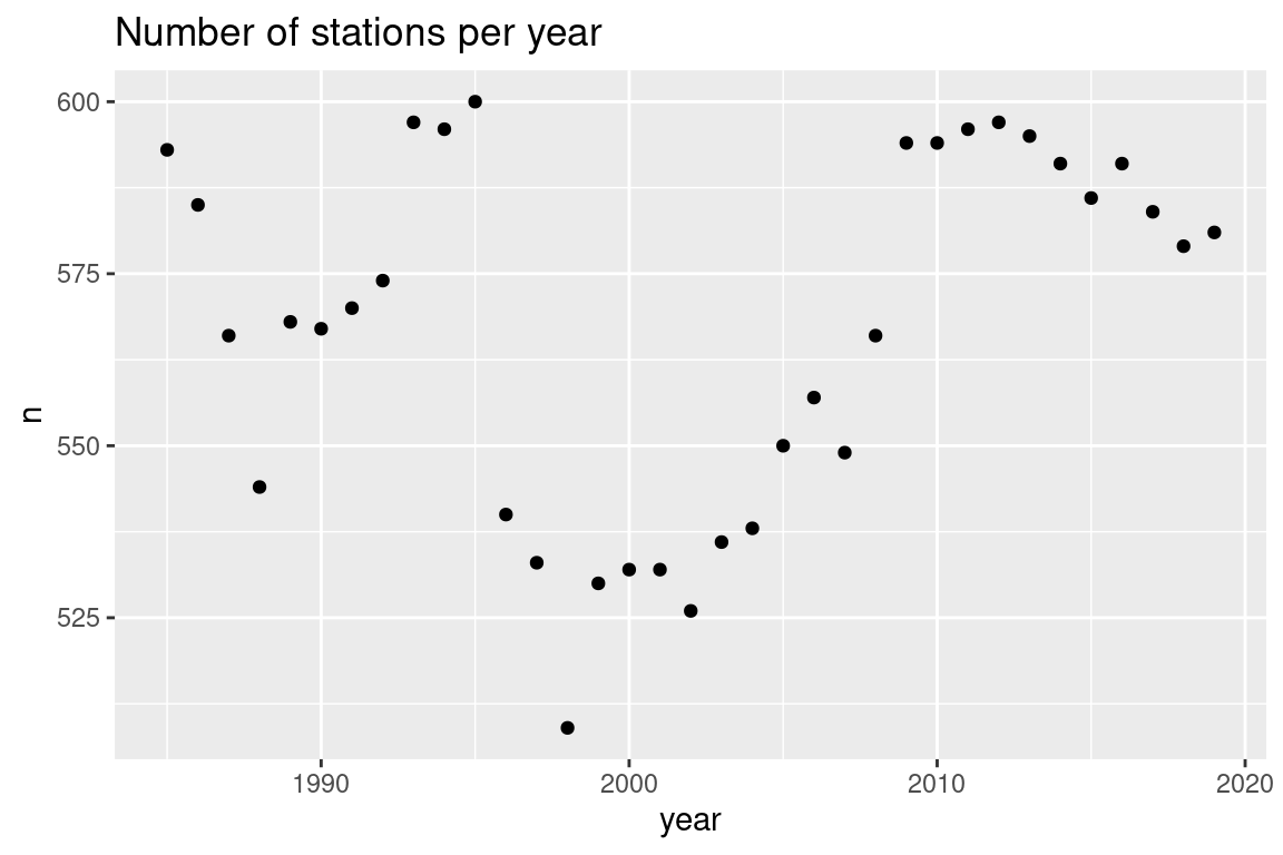
# Import -----------------------------------------------------------------------
library(tidyverse)
s <- 
  read_csv("ftp://ftp.hafro.is/pub/data/csv/is_smb_stations.csv")
b <- 
  read_csv("ftp://ftp.hafro.is/pub/data/csv/is_smb_biological.csv")
# Counts -----------------------------------------------------------------------

## Number of stations ----------------------------------------------------------

s |> 
  count(year) |> 
  ggplot(aes(year, n)) +
  geom_point() +
  labs(title = "Number of stations per year")

## When in year ----------------------------------------------------------------
s |>
  mutate(month = month(date)) |> 
  count(month)

# A tibble: 3 × 2
  month     n
  <dbl> <int>
1     2   544
2     3 19266
3     4    36

## What vessels ----------------------------------------------------------------
s |> 
  count(vid)

# A tibble: 16 × 2
     vid     n
   <dbl> <int>
 1  1131  1369
 2  1273  1160
 3  1274  1483
 4  1275  1248
 5  1276   118
 6  1277  3538
 7  1278  3458
 8  1279  1970
 9  1280  1282
10  1281   985
11  1307   976
12  1325   266
13  1459   199
14  1476   175
15  1976   178
16  2350  1441

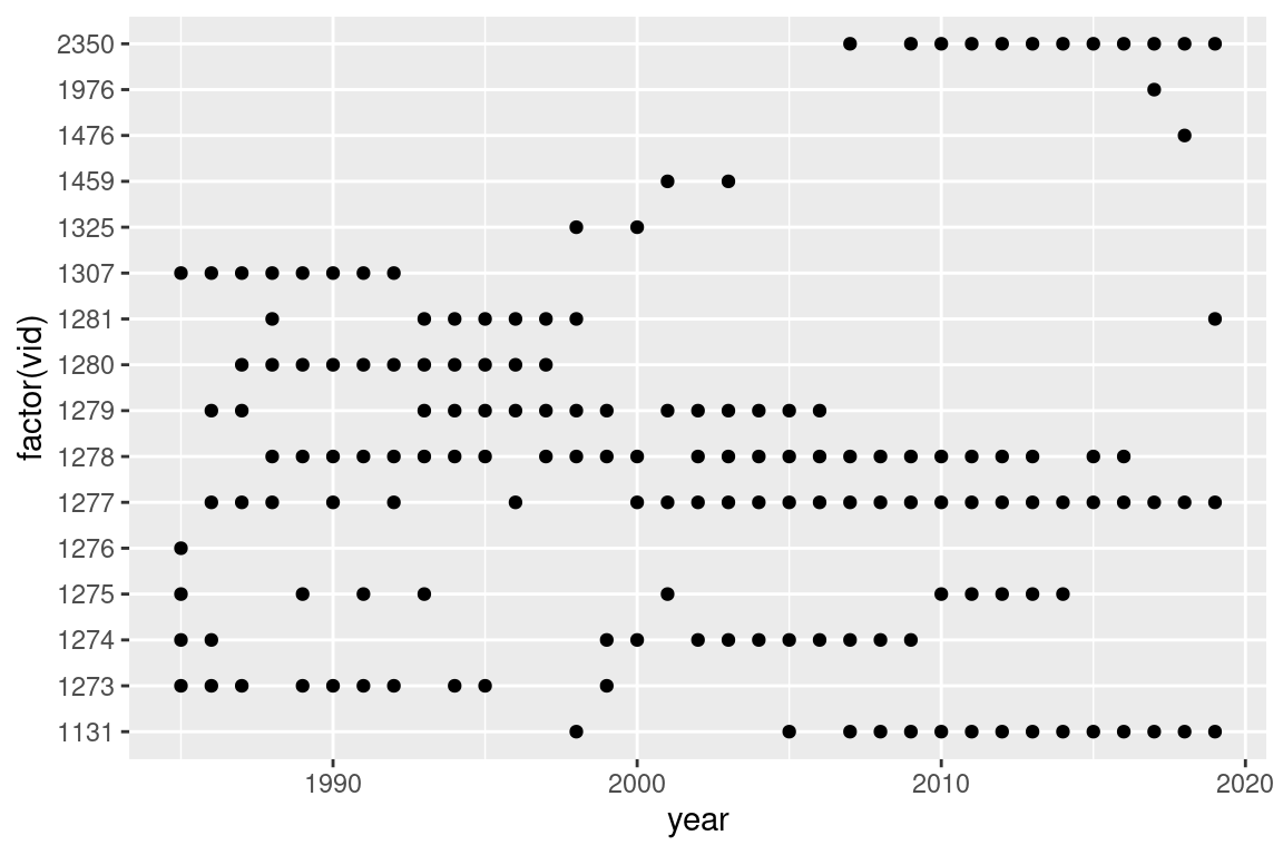
## When vessels ----------------------------------------------------------------
s |> 
  count(vid, year) |> 
  ggplot(aes(year, factor(vid))) +
  geom_point()

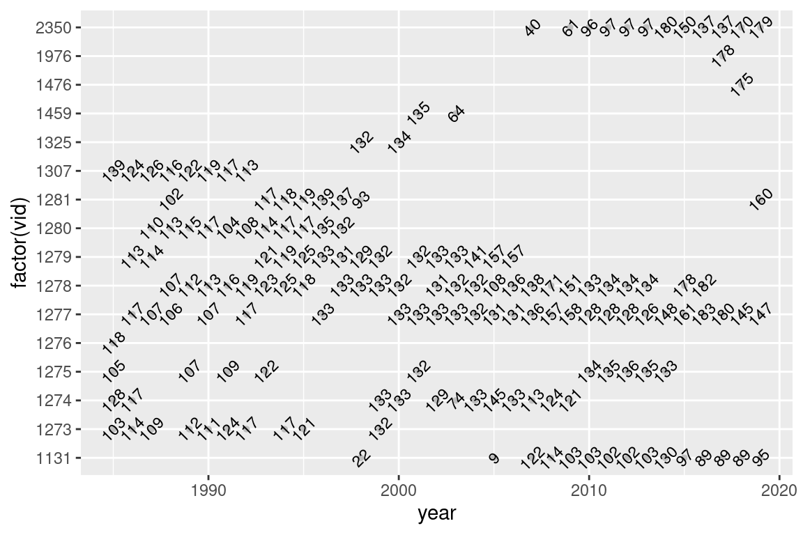
# Add informations on number of tows
s |> 
  count(vid, year) |> 
  ggplot(aes(year, factor(vid), label = n)) +
  geom_point(colour = "grey", size = 1) +   # size: control point size
  geom_text(angle = 45, size = 3)           # size: control text  size

# Distributions ----------------------------------------------------------------

## Towlength -------------------------------------------------------------------
s |> 
  ggplot(aes(towlength)) +
  geom_histogram()

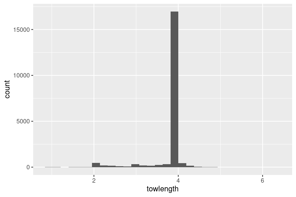
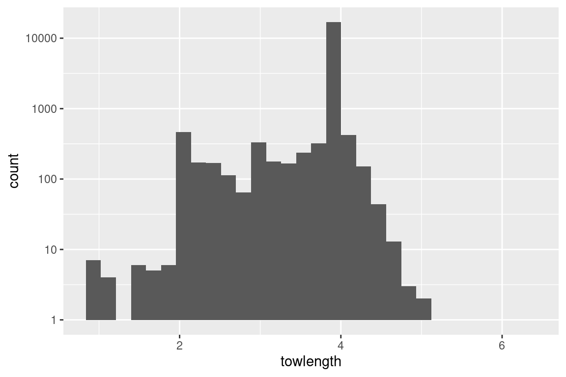
# change y-axis scale to get a better view of the smaller observations
s |> 
  ggplot(aes(towlength)) +
  geom_histogram() +
  scale_y_log10()

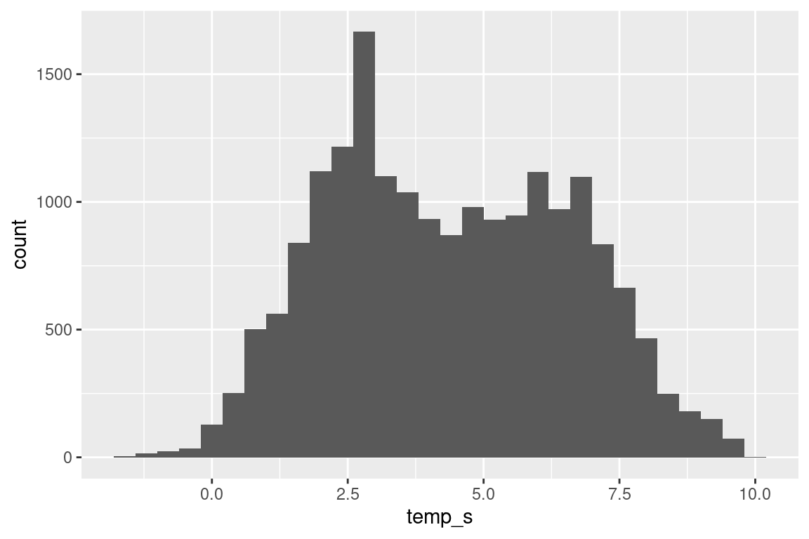
# what is the maximum towlength?
# max(s$towlength, na.rm = TRUE)  # 6.4
# Note: this maxmimum tow length does not show up in the histogram plots

## Temperature -----------------------------------------------------------------
# surface
s |> 
  ggplot(aes(temp_s)) +
  geom_histogram()

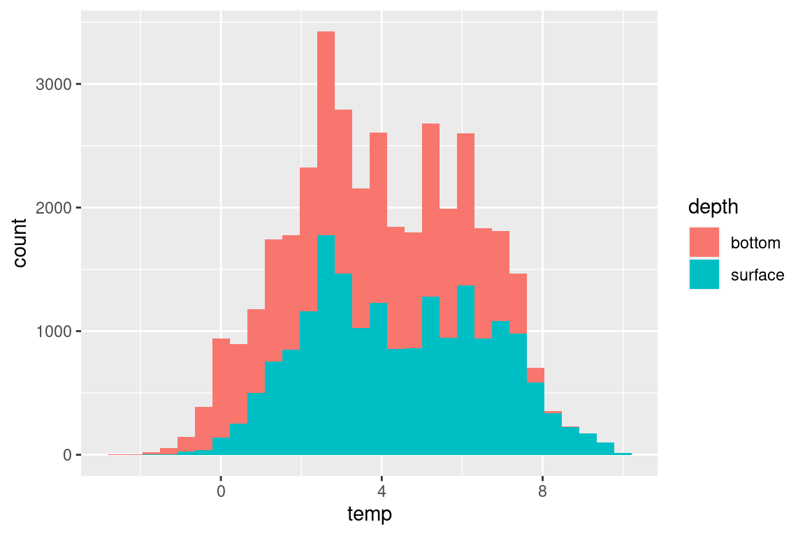
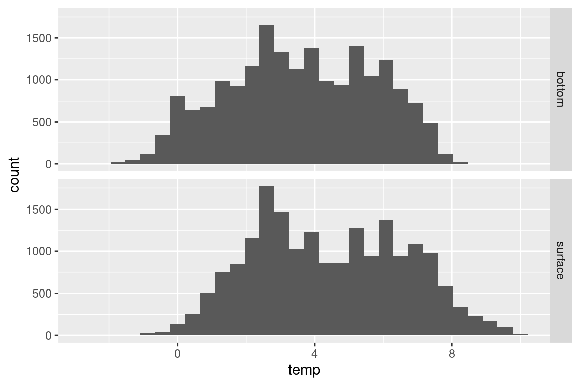
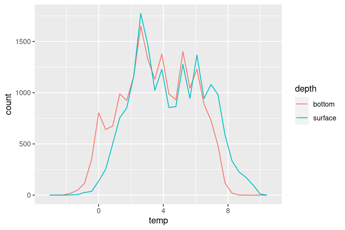
# both surface and bottom temperature
tmp <- 
  s |> 
  select(year, temp_s, temp_b) |> 
  pivot_longer(cols = temp_s:temp_b, names_to = "depth", values_to = "temp") |> 
  mutate(depth = case_when(depth == "temp_s" ~ "surface",
                           depth == "temp_b" ~ "bottom"))
tmp

# A tibble: 39,692 × 3
    year depth    temp
   <dbl> <chr>   <dbl>
 1  1990 surface   1.1
 2  1990 bottom   NA  
 3  1990 surface   1.1
 4  1990 bottom    1  
 5  1990 surface   1  
 6  1990 bottom   NA  
 7  1990 surface   1.1
 8  1990 bottom    1  
 9  1990 surface   0.9
10  1990 bottom    1.1
# ℹ 39,682 more rows

tmp |> 
  ggplot(aes(temp, fill = depth)) +
  geom_histogram()

# better
tmp |> 
  ggplot(aes(temp)) +
  geom_histogram() +
  facet_grid(depth ~ .)

# also better
tmp |> 
  ggplot(aes(temp, colour = depth)) +
  geom_freqpoly()

## Catch -----------------------------------------------------------------------
b |> 
  ggplot(aes(n)) +
  geom_histogram() +
  facet_wrap(~ species, scales = "free")

b |> 
  ggplot(aes(n)) +
  geom_histogram() +
  facet_wrap(~ species, scales = "free_y") +
  scale_x_log10()

# Correlations -----------------------------------------------------------------

## Temperatures ----------------------------------------------------------------
s |> 
  ggplot(aes(temp_s, temp_b)) +
  geom_point(alpha = 0.1) +      # alpha controls transparency, range 0-1
  geom_smooth()

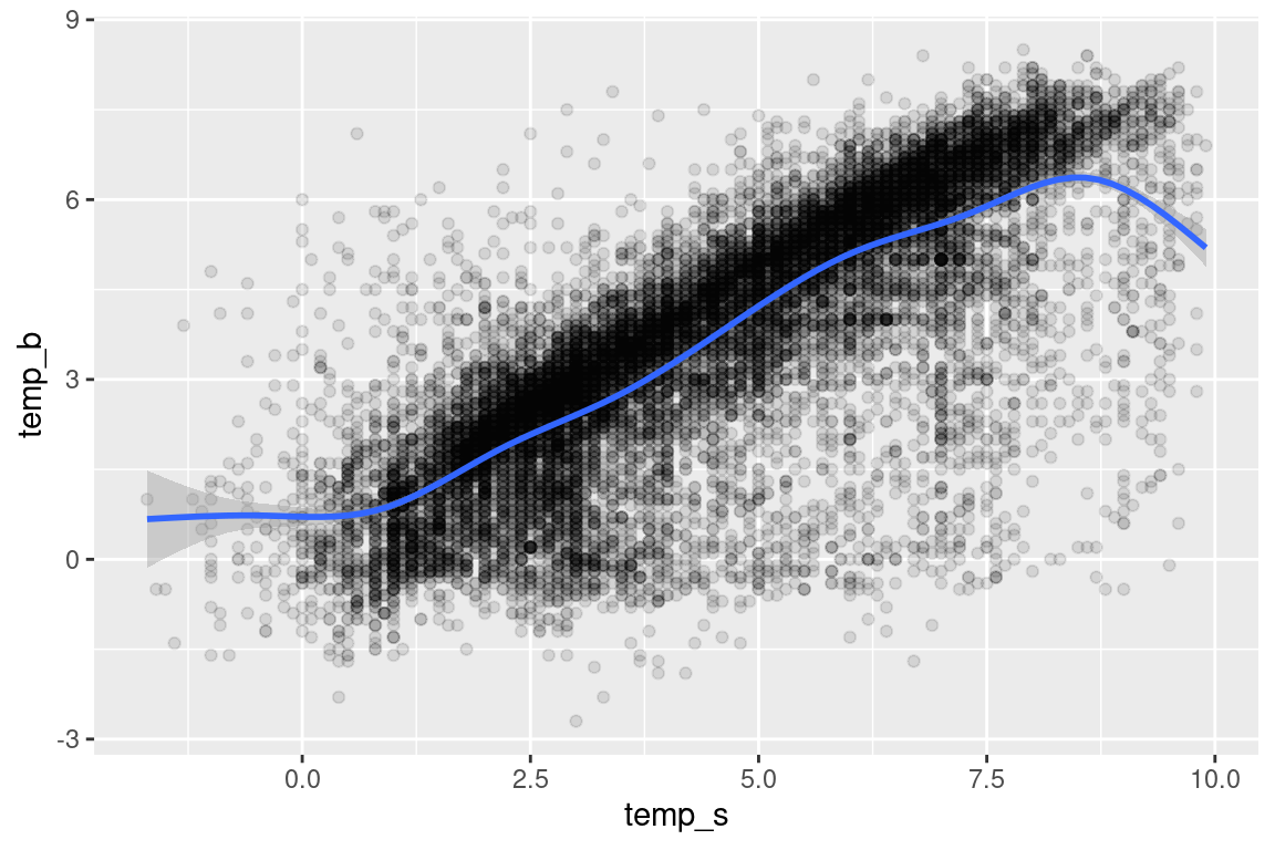
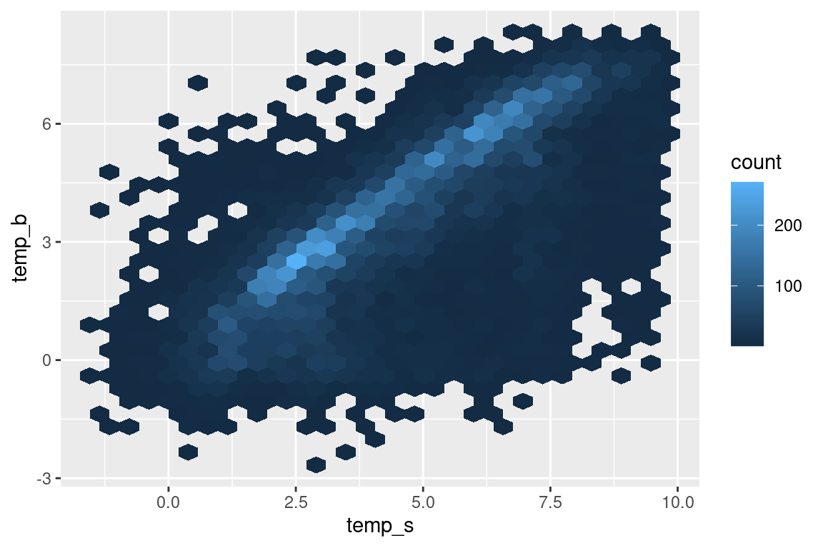
s |> 
  ggplot(aes(temp_s, temp_b)) +
  geom_hex()  # geom_hex provides number of observations within bins

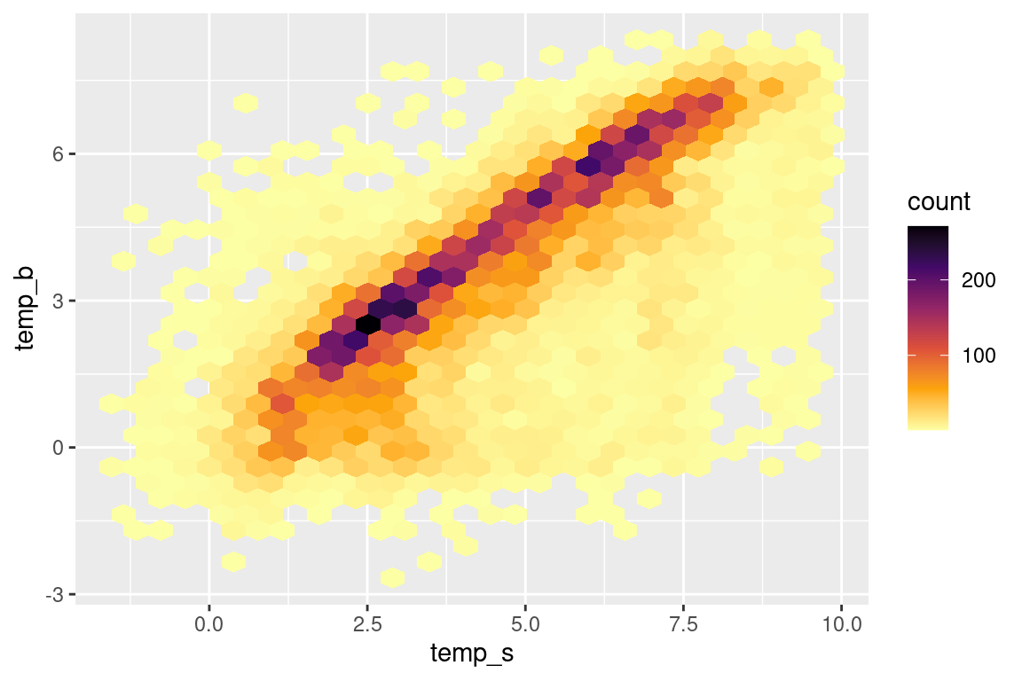
# overwrite the default colour
s |> 
  ggplot(aes(temp_s, temp_b)) +
  geom_hex() +
  scale_fill_viridis_c(option = "B", direction = -1)

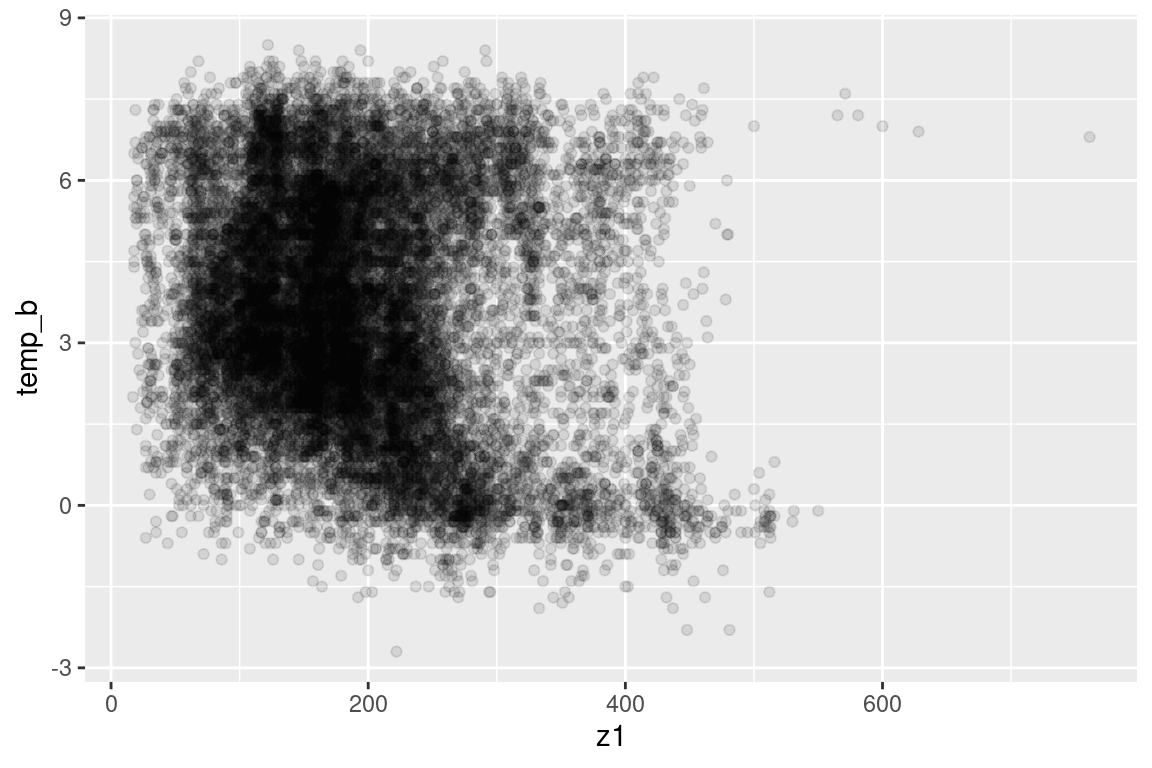
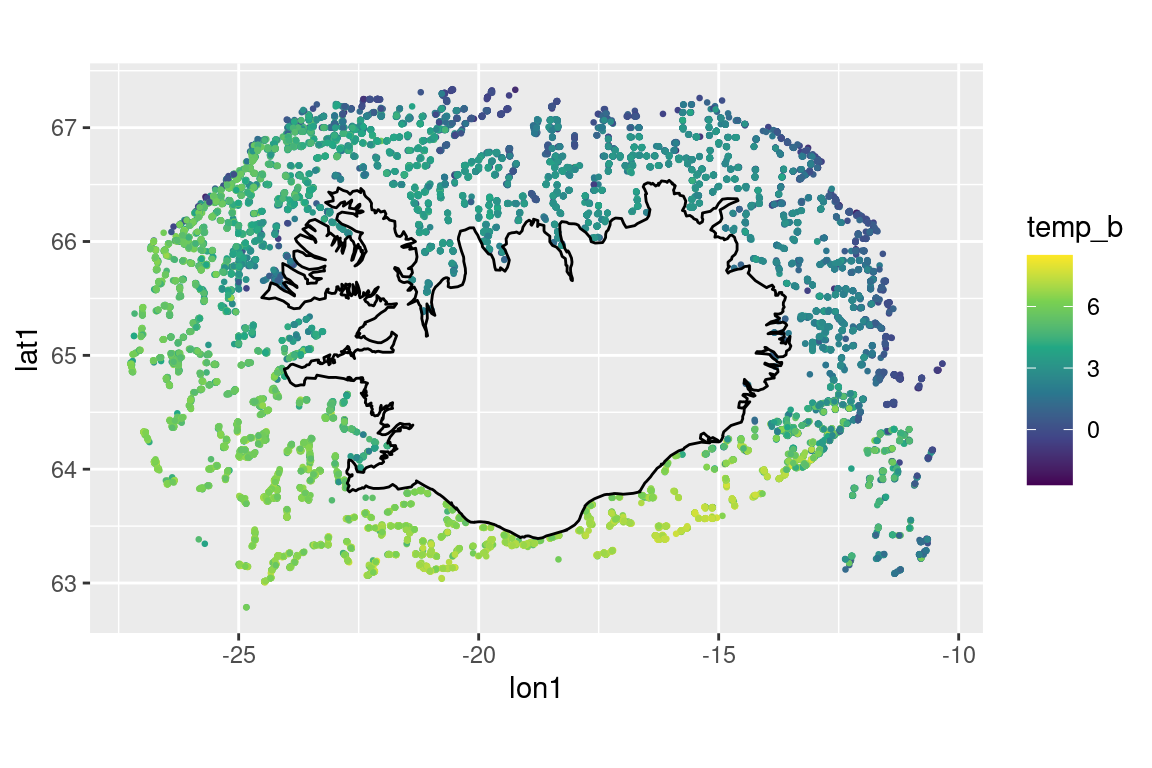
## Temperature vs depth --------------------------------------------------------
s |> 
  ggplot(aes(z1, temp_b)) +
  geom_point(alpha = 0.1)

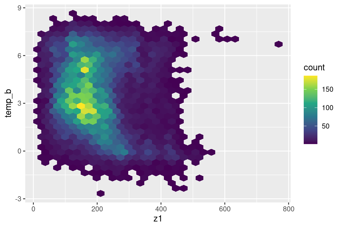
s |> 
  ggplot(aes(z1, temp_b)) +
  geom_hex() +
  scale_fill_viridis_c()

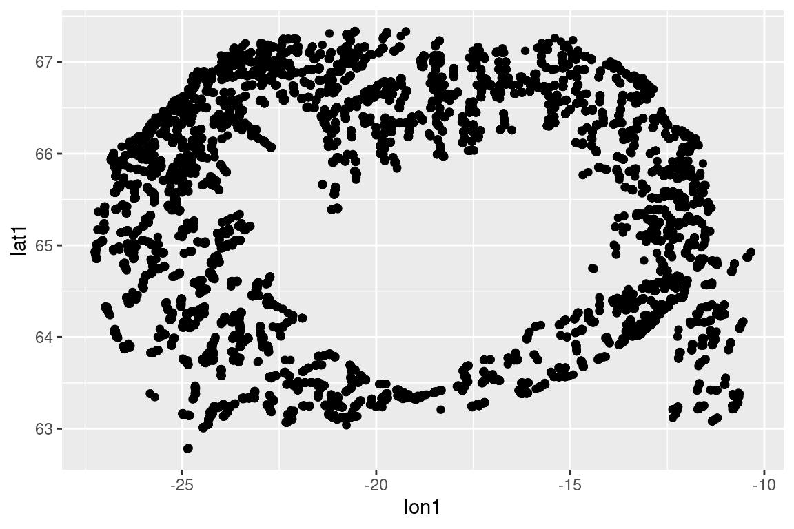
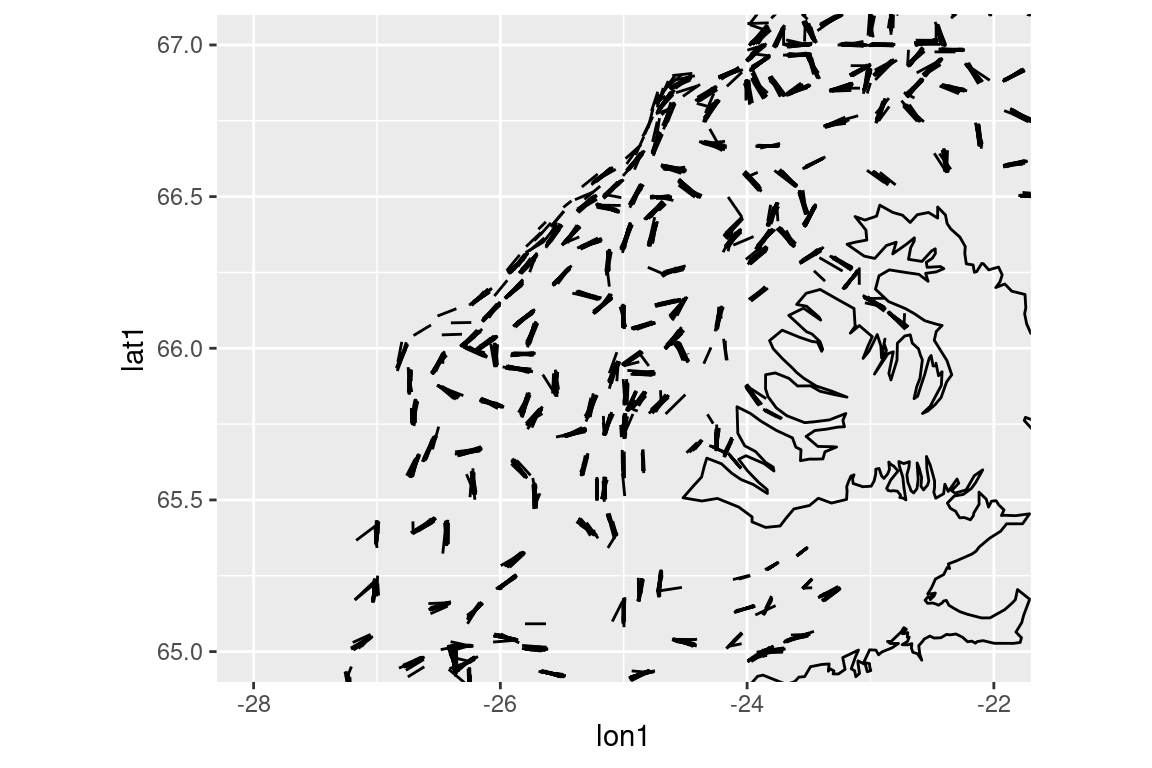
# Spatial stuff ----------------------------------------------------------------

## Tow locations ----------------------------------------------------------------

# Just the starting point
s |> 
  ggplot(aes(lon1, lat1)) +
  geom_point()

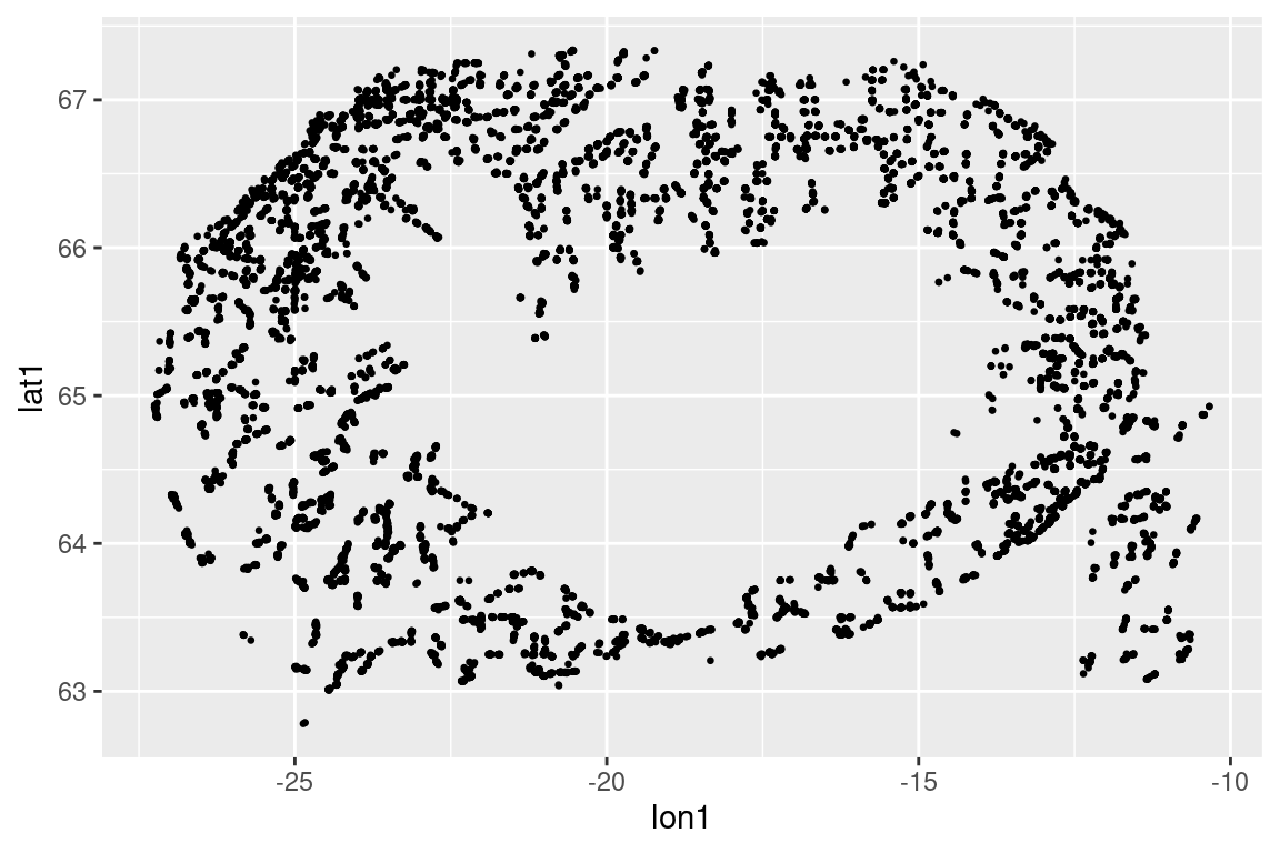
# Get the aspect ratio roughly right
s |> 
  ggplot(aes(lon1, lat1)) +
  geom_point(size = 0.5) +
  coord_quickmap()

# zoom in
s |> 
  ggplot(aes(lon1, lat1)) +
  geom_point(size = 0.5) +
  coord_quickmap(xlim = c(-28, -25),
                 ylim = c( 65,  67))

# add some reference lines
ice = read_csv("https://heima.hafro.is/~einarhj/data/island.csv")
s |> 
  ggplot(aes(lon1, lat1)) +
  geom_point(size = 0.5) +
  geom_path(data = ice,
            aes(lon, lat)) +
  coord_quickmap(xlim = c(-28, -22),
                 ylim = c( 65,  67))

## actual tow tracks -----------------------------------------------------------
s |> 
  ggplot(aes(lon1, lat1)) +
  geom_segment(aes(x = lon1, y = lat1, 
                   xend = lon2, yend = lat2)) +
  geom_path(data = ice,
            aes(lon, lat)) +
  coord_quickmap(xlim = c(-28, -22),
                 ylim = c( 65,  67))

## Spatial temperature distribution --------------------------------------------
s |> 
  filter(!is.na(temp_b)) |> 
  ggplot(aes(lon1, lat1)) +
  geom_point(aes(colour = temp_b), size = 0.5) +
  geom_path(data = ice, 
            aes(lon, lat)) +
  scale_colour_viridis_c() +
  coord_quickmap()

## Species distribution --------------------------------------------------------
s |> 
  filter(year == 2012) |> 
  select(id, lon1, lat1) |> 
  left_join(b) |> 
  filter(species == "cod") |> 
  ggplot() +
  geom_point(aes(lon1, lat1, size = n), 
             colour = "red", alpha = 0.5) +
  scale_size_area(max_size = 10) +
  facet_wrap(~ species) +
  coord_quickmap()

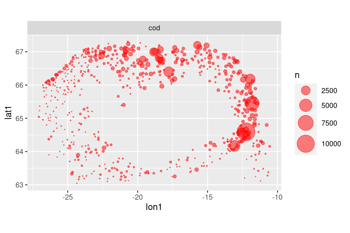
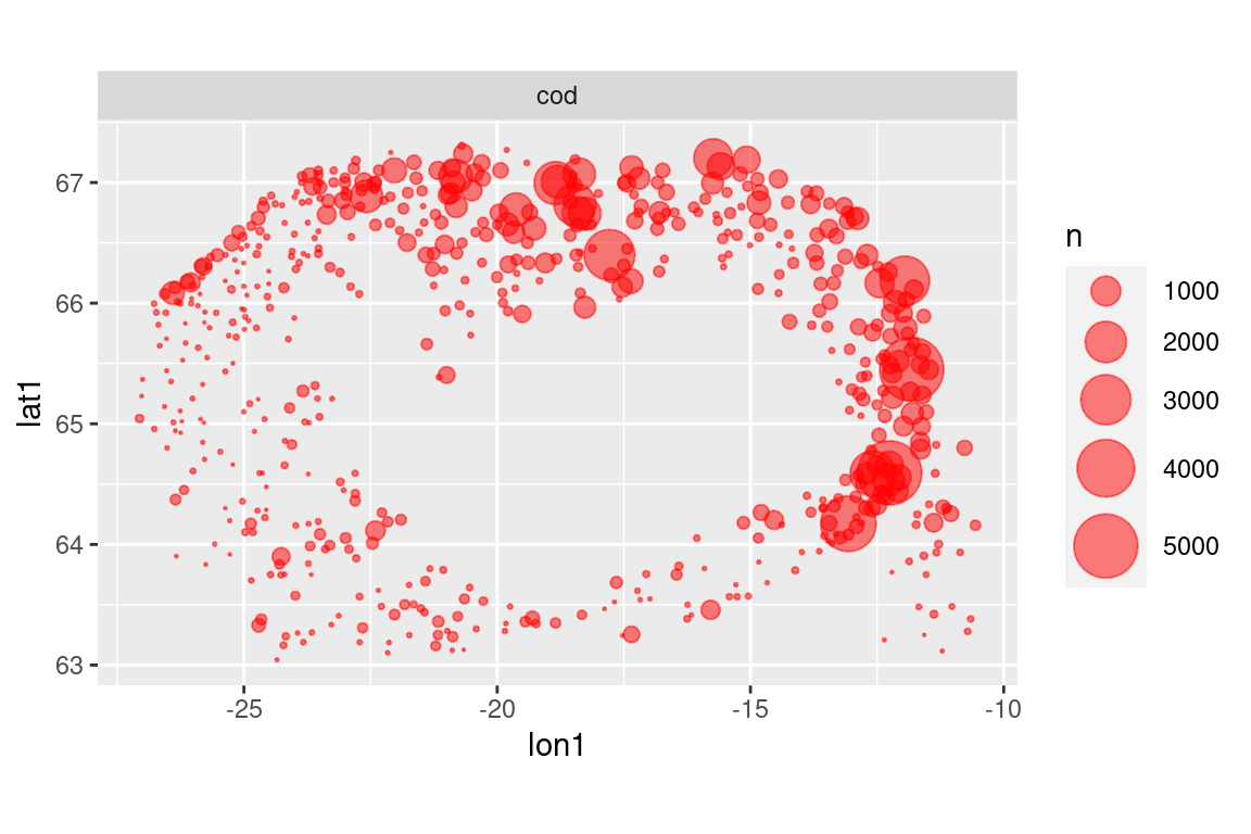
# put some upper cap on data
s |> 
  filter(year == 2012) |> 
  select(id, lon1, lat1) |> 
  left_join(b) |> 
  filter(species == "cod") |> 
  mutate(n = ifelse(n > 5000, 5000, n)) |> 
  ggplot() +
  geom_point(aes(lon1, lat1, size = n), 
             colour = "red", alpha = 0.5) +
  scale_size_area(max_size = 10) +
  facet_wrap(~ species) +
  coord_quickmap()

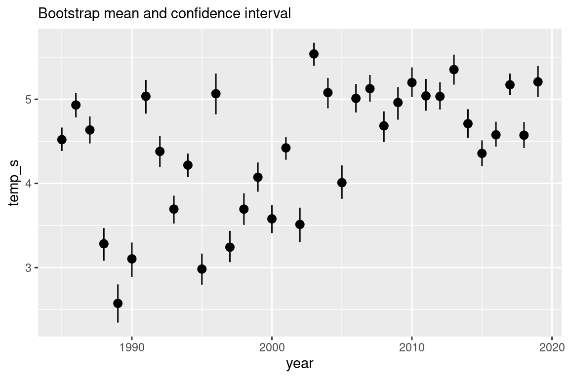
# Summary geoms ---------------------------------------------------------------

## Surface temperature over time -----------------------------------------------
s |> 
  filter(!is.na(temp_s)) |> 
  ggplot(aes(year, temp_s)) +
  stat_summary(fun.data = "mean_cl_boot") +
  labs(subtitle = "Bootstrap mean and confidence interval")

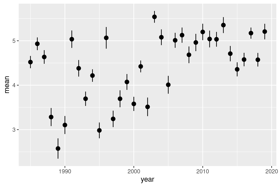
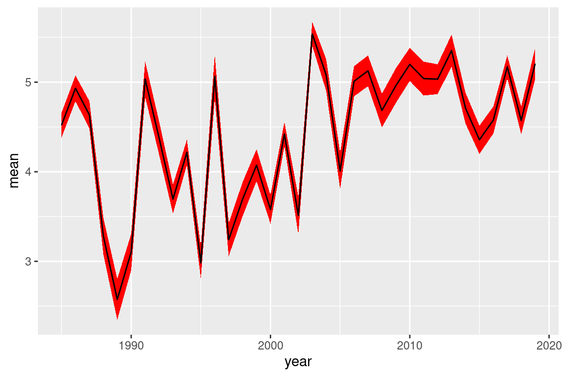
# could also do
tmp <- 
  s |> 
  filter(!is.na(temp_s)) |> 
  group_by(year) |> 
  summarise(n = n(),
            mean = mean(temp_s, na.rm = TRUE),
            sd = sd(temp_s, na.rm = TRUE),
            se = sd / sqrt(n))
tmp

# A tibble: 35 × 5
    year     n  mean    sd     se
   <dbl> <int> <dbl> <dbl>  <dbl>
 1  1985   503  4.52  1.58 0.0705
 2  1986   577  4.93  1.75 0.0730
 3  1987   560  4.64  1.85 0.0783
 4  1988   540  3.28  2.42 0.104 
 5  1989   459  2.57  2.50 0.116 
 6  1990   542  3.10  2.41 0.104 
 7  1991   553  5.04  2.35 0.100 
 8  1992   559  4.38  2.25 0.0950
 9  1993   589  3.70  2.00 0.0823
10  1994   595  4.22  1.75 0.0719
# ℹ 25 more rows

tmp |> 
  ggplot() +
  geom_pointrange(aes(x = year, 
                      y = mean, 
                      ymin = mean - 1.96 * se, 
                      ymax = mean + 1.96 * se)) 

tmp |> 
  ggplot() +
  geom_ribbon(aes(x = year, 
                  ymin = mean - 1.96 * se, 
                  ymax = mean + 1.96 * se),
              fill = "red") +
  geom_line(aes(x = year, y = mean))

## Trends in cod cpue ----------------------------------------------------------
s |> 
  select(id, year) |> 
  left_join(b |> filter(species == "cod")) |> 
  mutate(kg = replace_na(kg, 0)) |>
  ggplot(aes(year, kg)) +
  stat_summary(fun.data = "mean_cl_boot") +
  labs(title = "Cod: Catch per unit effort",
       subtitle = "Bootstrap mean and confidence interval")