A workflow model

Points assigned to squares

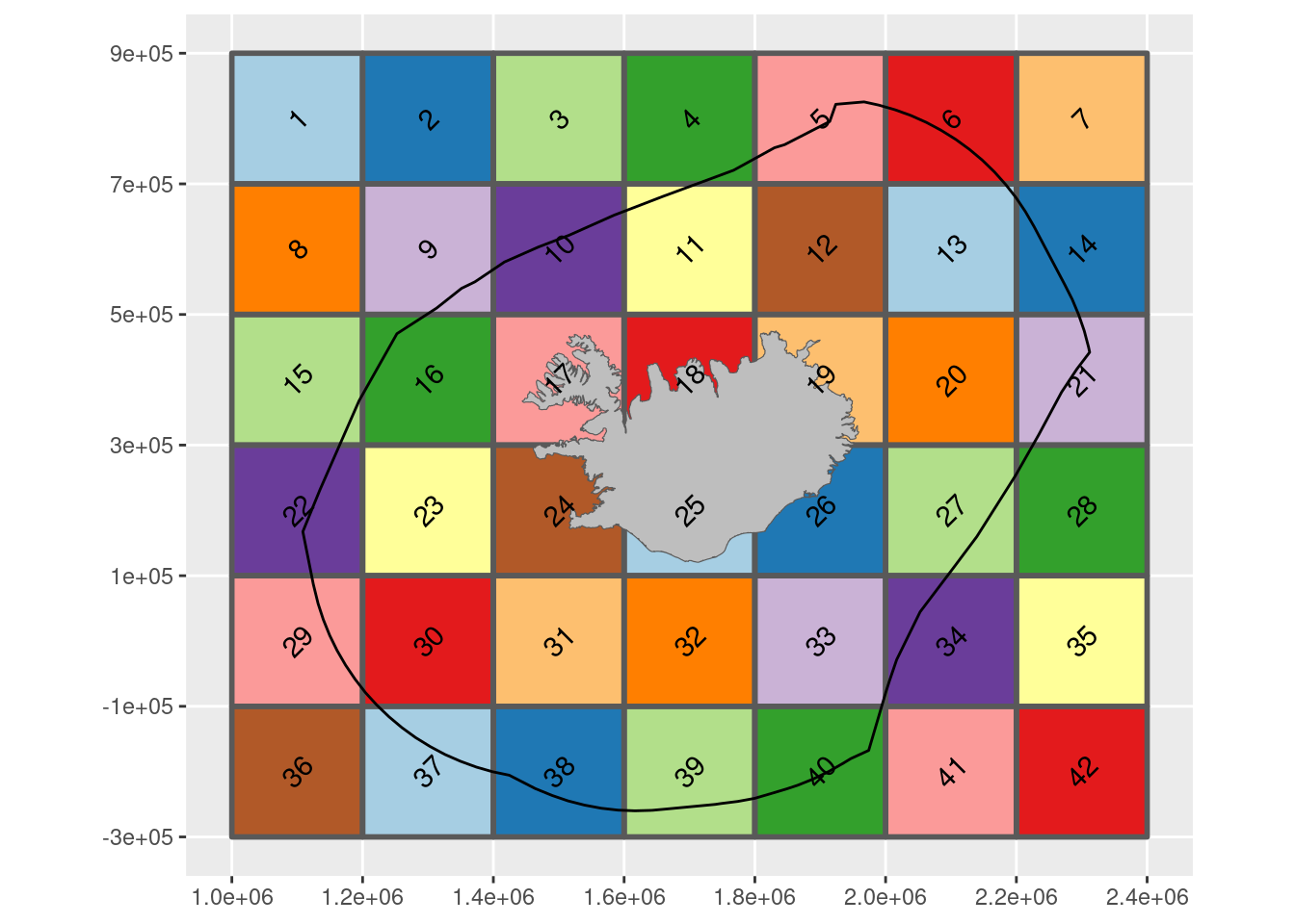
In the data compilation of xyz-data into parquet files each ping is for convenience assigned to a particular square according to the following grid-model:

library(terra)
library(tidyterra)
library(tidyverse)
library(arrow)
library(sf)
CRS <- 5325
eez <- 
  gisland::read_eez() |> 
  st_transform(crs = CRS)
island <-
  geo::bisland |> 
  st_as_sf(coords = c("lon", "lat"),
           crs = 4326) |> 
  st_transform(crs = CRS) |> 
  summarise(do_union = FALSE) |> 
  st_cast("LINESTRING") |> 
  st_cast("POLYGON")

bb <- c(1e6, 2.4e6, -3e5, 9e5)
r <-
  terra::rast(xmin = bb[1],
              xmax = bb[2],
              ymin = bb[3],
              ymax = bb[4],
              nlyrs = 1,
              resolution = c(8, 8),
              crs = paste0("epsg:", CRS))
dr <- ceiling(nrow(r) * 8 / 2e5)  # a band of 2e5 meters
dc <- ceiling(ncol(r) * 8 / 2e5)  # a band of 2e5 meters
dr  <- ceiling(nrow(r) / dr)
dc  <- ceiling(ncol(r) / dc)
agg <- terra::aggregate(r, fact = c(dr, dc))
values(agg) <-  as.factor(1:(nrow(agg) * ncol(agg)))
pts <- 
  terra::crds(agg, df = TRUE) |> 
  as_tibble() |> 
  mutate(sq = values(agg))
po <- terra::as.polygons(agg)
values(po) <- NA
ggplot() +
  geom_spatraster(data = agg) +
  geom_spatvector(data = po, alpha = 0, lwd = 1) +
  geom_sf(data = eez) +
  geom_sf(data = island, fill = "grey") +
  geom_text(data = pts, aes(x, y, label = sq),
            angle = 45) +
  ggmisc::scale_fill_crayola() +
  coord_sf(crs = CRS, datum = CRS) +
  scale_x_continuous(NULL, seq(1e6, 3e6, 2e5), labels = scales::scientific) +
  scale_y_continuous(NULL, seq(-3e5, 9e5, 2e5), labels = scales::scientific)

agg |> 
  terra::as.polygons() |> 
  st_as_sf() |> 
  rename(sq = 1) |>
  mutate(sq = as.integer(sq)) |> 
  write_sf("data/m_squares.gpkg")

One could even entertain assigning each observation to a 8x8 meter raster. Then reasterization could be done from within parquet. But then how should one go if the raster of interest is e.g. 32x32 meters?

A “dynamic raster”

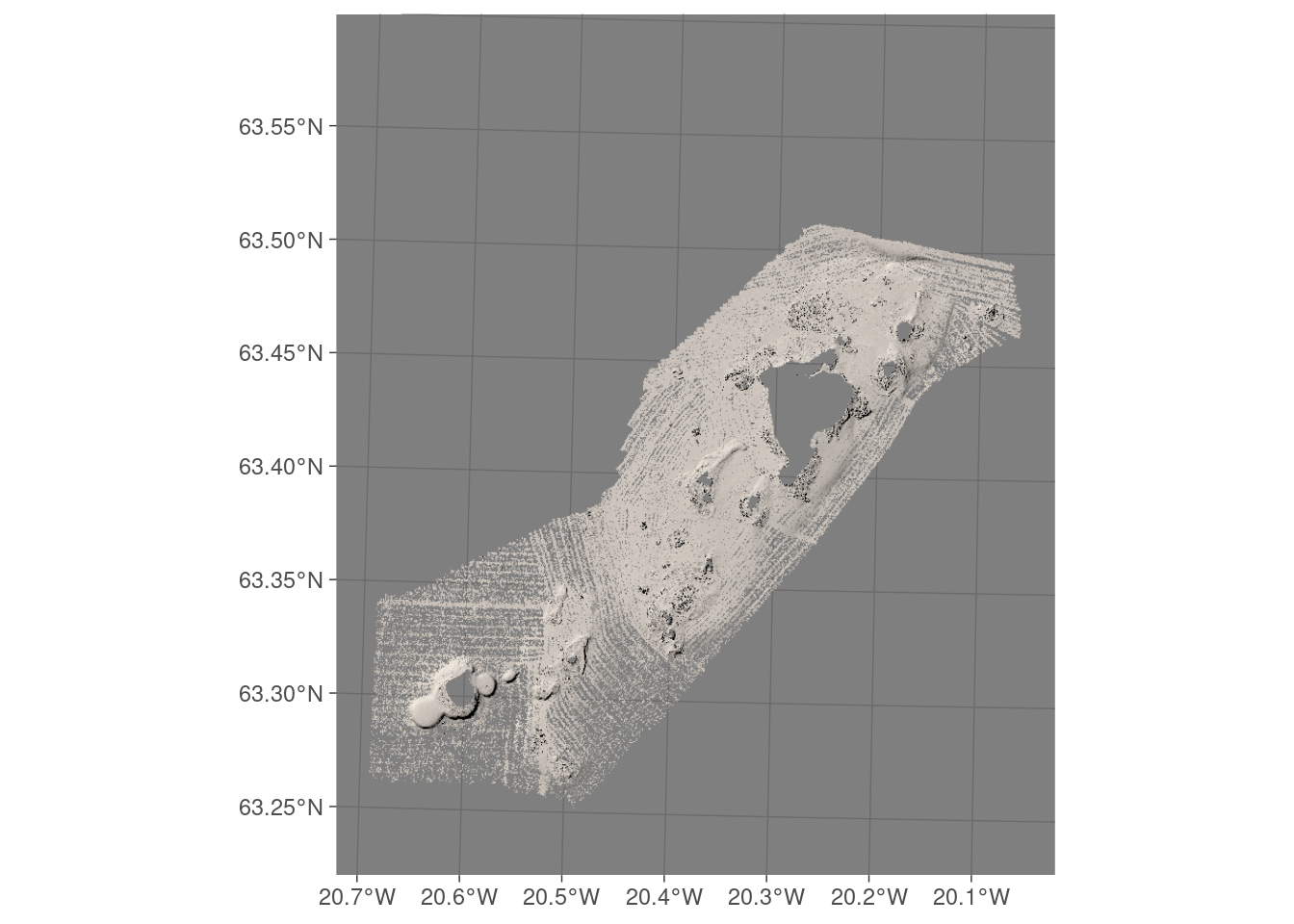
An attemp was made to create rayshade-model of bathymetric relief using a “dynamic” rasterization. In principle the process was to generate rayshades first at 8x8 meter resolution, next 16x16 meter, then 32x32 meters, 64x64 meters ending with 128x128 meters. At each level of rasterization a criteria was used such that if the observations points were less than 10 no rayshading was done at that level. The choice of less than 10 is arbritrary and a better approach may need to be thought of.

Quick and dirty rastering within arrow

We can do a poor-man’s rasterization within parquet quite easily via:

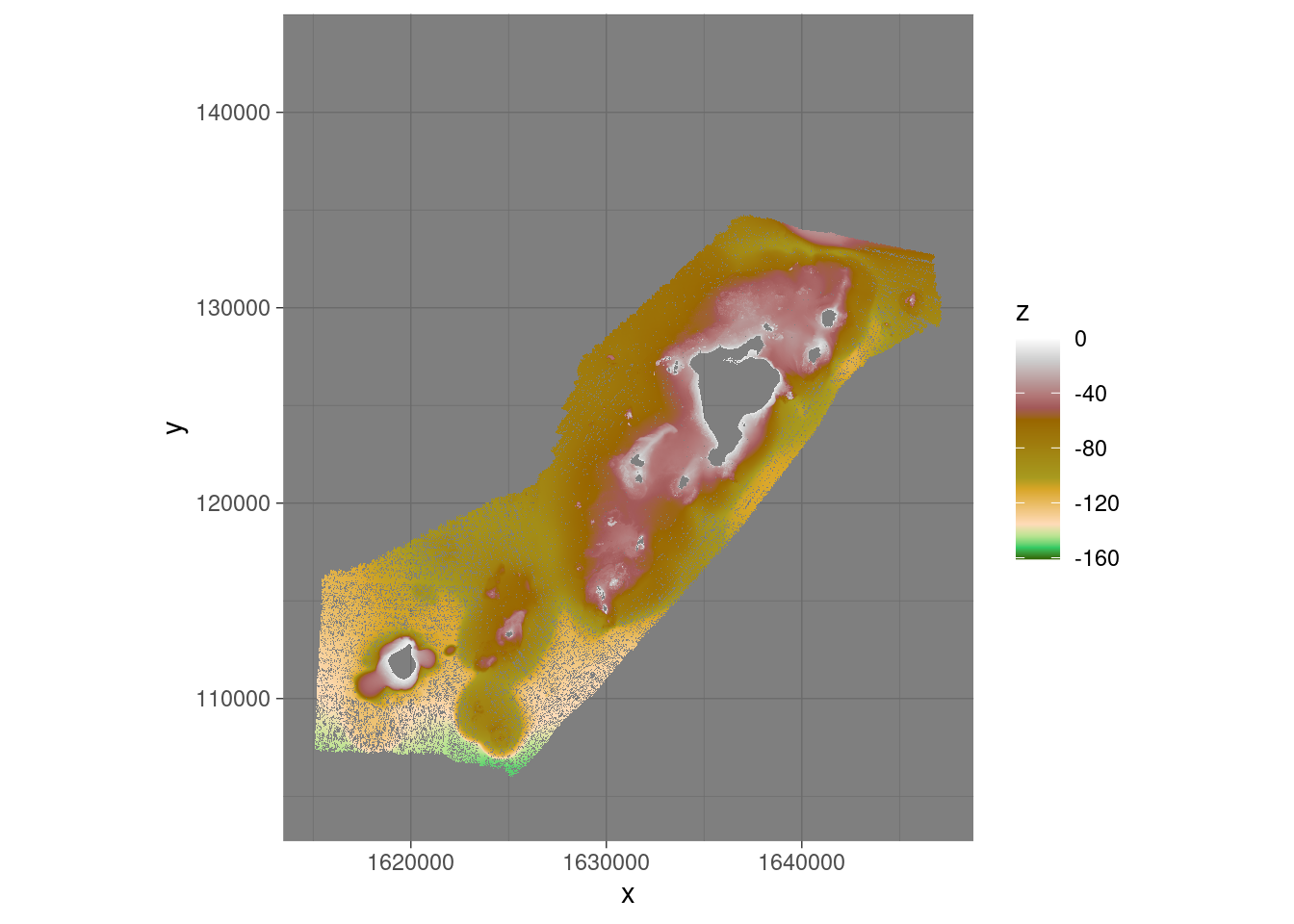
con <- open_dataset("/net/hafkaldi.hafro.is/export/home/haf/einarhj/stasi/gis/botninn/data-parquet/xyz")
dx <- 5  # the grid resolution in meters
g <- 
  con |>
  filter(sq == 25) |> 
  mutate(x = x %/% dx * dx + dx/2,
         y = y %/% dx * dx + dx/2,
         one = 1L) |> 
  group_by(x, y) |> 
  summarise(n = sum(one),
            z = mean(z),
            .groups = "drop") |> 
  # at minimum 3 pings (read: measurements) per grid
  filter(n > 2) |> 
  select(x, y, z) |> 
  collect()
g |> glimpse()

Rows: 13,319,928
Columns: 3
$ x <dbl> 1638778, 1638782, 1638788, 1638792, 1638798, 1638712, 1638768, 16387…
$ y <dbl> 127507.5, 127507.5, 127507.5, 127507.5, 127507.5, 127512.5, 127522.5…
$ z <dbl> -45.08563, -45.02414, -44.88000, -44.80667, -44.74017, -45.58057, -4…

ggplot() +
  theme_dark() +
  geom_tile(data = g,
            aes(x, y, fill = z)) +
  scale_fill_hypso_c() +
  coord_equal()

r <- 
  terra::rast(x = g, type = "xyz",
              crs = paste0("epsg:", CRS)) |> 
  terra::trim()
ggplot() +
  geom_spatraster(data = r) +
  scale_fill_hypso_c()

rs <-
  r |> 
  ramb::mb_rayshade_raster_rgb(zscale = 1)

[1] "Number of tiles: 4"

ggplot() +
  theme_dark() +
  geom_spatraster_rgb(data = rs)

library(tmap)
tmap_mode("view")
tmap_options(max.raster = c(plot = 1e6, view = 2e6))
#tmap_options(raster.max.cells = 27014160) #7696 * 6421
tm_basemap("CartoDB.DarkMatter") +
  tm_shape(rs, ) +
  tm_rgb(r=1, g=2, b=3)

  #tm_rgb(col = tm_vars(c(1, 2, 3), multivariate = TRUE))

Now it is obvious from the above that we have some gaping holes at this resolution, those being related to the depth. If one were interested in only the most “data-rich” regions we would/could limit the bounds.

Poor-mans dynamic raster

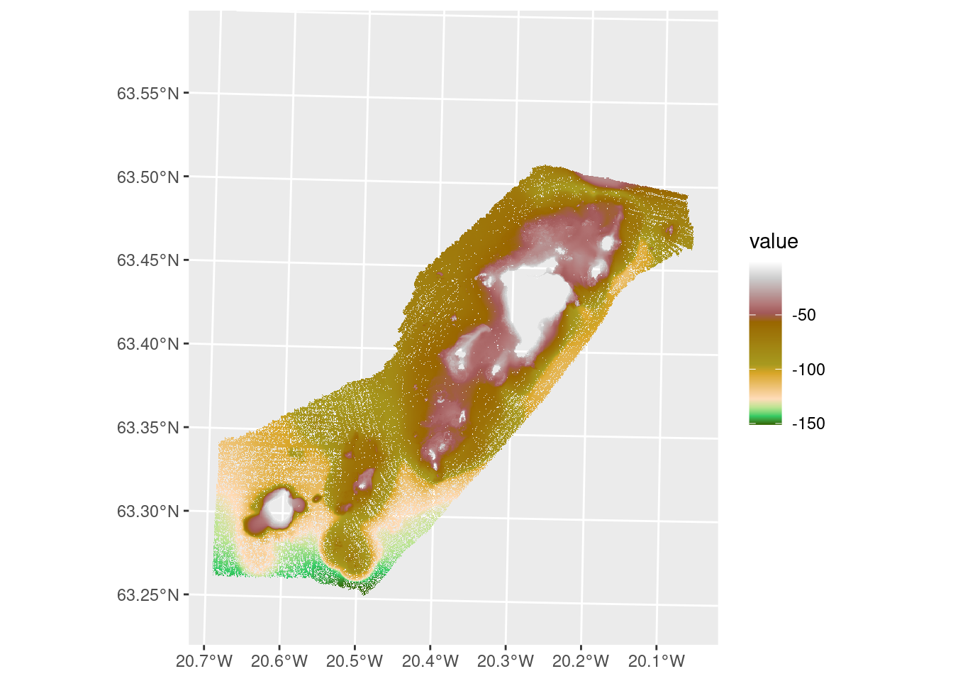
Another way is some kind of a dynamic rastering/rayshading as described above. Here is one code-take on achieving that using “dynamic” rastering:

# NOT RUN
dx <- 5  # milking the stone
xyz <- 
  con |>
  filter(sq == 25,
         # trim some "outliers"
         x < 1.65e6,
         y < 1.35e5) |> 
  mutate(x = x %/% dx * dx + dx/2,
         y = y %/% dx * dx + dx/2) |> 
  group_by(x, y) |> 
  summarise(z = mean(z),
            .groups = "drop") |> 
  collect()

r0 <-
  xyz |> 
  terra::rast(type = "xyz",
              crs = paste0("epsg:", CRS)) |> 
  terra::trim()
# this takes a while (for now, at least) ...
rs <- 
  ramb::mb_rashade_xyz_dynamic(xyz, r0, file_prefix = "tmp/vestmannaeyjar_")
rs |> terra::writeRaster("tmp_vestmannaeyjar.tif")
# create png tiles, for demo. no downsampling here
tiler::tile(file = "tmp_vestmannaeyjar.tif",
             zoom = "0-15",
             tiles = "/net/hafri.hafro.is/export/home/hafri/einarhj/public_html/tiles/vestmannaeyjar")
system("chmod -R a+rx /net/hafri.hafro.is/export/home/hafri/einarhj/public_html/tiles/vestmannaeyjar")

Get a view of the tiled results one could do:

library(leaflet)
leaflet() %>%
  setView(lng = -20.4,
          lat =  63.35,
          zoom =  9) %>%
  addTiles(urlTemplate = "https://server.arcgisonline.com/ArcGIS/rest/services/World_Imagery/MapServer/tile/{z}/{y}/{x}",
           #group = "Hnöttur",
           attribution = 'Data source: <a href="https://www.hafogvatn.is">Marine & Freshwater Research Institute</a>') |>
    addTiles(urlTemplate = "https://heima.hafro.is/~einarhj/tiles/vestmannaeyjar/{z}/{x}/{-y}.png",
             group = "vestmannaeyjar",
             options = tileOptions(minZoom = 0, maxZoom = 14))

tmap              * 3.99.9002  2024-08-25 [1] Github (r-tmap/tmap@e7aa29a)