Cleaning data

Preamble

The difference between tidying vs cleaning:

Tidying refers to restructuring the dataset such that each column is a variable and each row an observation.
Cleaning refers to changing values in a variable, most often because of data-entry mistakes.

In this session we are going to read in some catch sampling data from a country and a specific period. The data structure is tidy but there are various issues with the data entry. Each record (row) consist of the following observations:

vessel id
landing site id
date of sampling
gear id
species id
catch weight (these have been scrambled)

The data collection at the landings site were initially recorded on a paper and then entered in a spreadsheet in the office. This is a very common procedure. Also what is most common is that there were no restrictions made with respect to what could be entered in the spreadsheet.

Import

library(tidyverse)
library(janitor)

d <- 
  read_csv("https://heima.hafro.is/~einarhj/data/raw-data.csv",
           # this argument is to ensure that the function read_csv is not guessing the variable
           #  type from the first 100 thousand records
           guess_max = Inf)

New names:
Rows: 14966 Columns: 16
── Column specification
──────────────────────────────────────────────────────── Delimiter: "," chr
(7): Vessel #, LANDING SITE, DATE MM/DD/YYYY, GEAR, SPECIES, SOAK TIM... dbl
(2): WEIGHT...6, TRAPS PULL lgl (7): WEIGHT...10, Fishing 1, Fishing2,
Fishing3, PAB, Fdays, Raised
ℹ Use `spec()` to retrieve the full column specification for this data. ℹ
Specify the column types or set `show_col_types = FALSE` to quiet this message.
• `WEIGHT` -> `WEIGHT...6`
• `WEIGHT` -> `WEIGHT...10`

Initially when we read in any data it is important to read the messages that we obtain. When using read_csv we get some informations about what type each variable is allocated to (like “chr”, “dbl” and “lgl”). Also here we get the information that the column name “WEIGHT” occurs twice. And because in R we can not have the same variable name twice in a dataframe, read_csv adds “…X” to the original, the X being a number that denotes in what column number in the original data each of the duplicate names occurs (here column number 6 and 10).

Lets get a peak at the data:

d |> glimpse()

Rows: 14,966
Columns: 16
$ `Vessel #`           <chr> "586BE", "586BE", "428SP", "428SP", "586BE", "586…
$ `LANDING SITE`       <chr> "BAEP", "BAEP", "SAPB", "SAPB", "BAEP", "BAEP", "…
$ `DATE    MM/DD/YYYY` <chr> "01/01/2023", "01/01/2023", "01/01/2023", "01/01/…
$ GEAR                 <chr> "SGUN", "SGUN", "HLIN", "HLIN", "SGUN", "SGUN", "…
$ SPECIES              <chr> "CLASSD", "PALIAR", "SERRGU", "SERRFU", "CLASSD",…
$ WEIGHT...6           <dbl> 5, 240, 155, 20, 4, 85, 10, 10, 14, 22, 12, 12, 5…
$ `TRAPS PULL`         <dbl> NA, NA, NA, NA, NA, NA, 200, 200, 200, NA, NA, NA…
$ `SOAK TIME  (HRS)`   <chr> NA, NA, NA, NA, NA, NA, "14", "14", "14", NA, NA,…
$ `AREA FISHED`        <chr> "E7", "E7", "B3", "B3", "E7", "E7", "D3,E3,D4,E4"…
$ WEIGHT...10          <lgl> NA, NA, NA, NA, NA, NA, NA, NA, NA, NA, NA, NA, N…
$ `Fishing 1`          <lgl> NA, NA, NA, NA, NA, NA, NA, NA, NA, NA, NA, NA, N…
$ Fishing2             <lgl> NA, NA, NA, NA, NA, NA, NA, NA, NA, NA, NA, NA, N…
$ Fishing3             <lgl> NA, NA, NA, NA, NA, NA, NA, NA, NA, NA, NA, NA, N…
$ PAB                  <lgl> NA, NA, NA, NA, NA, NA, NA, NA, NA, NA, NA, NA, N…
$ Fdays                <lgl> NA, NA, NA, NA, NA, NA, NA, NA, NA, NA, NA, NA, N…
$ Raised               <lgl> NA, NA, NA, NA, NA, NA, NA, NA, NA, NA, NA, NA, N…

Variable names

I usually look at the variable names first, and here I just do not like them. In general:

Long names makes coding downstream problematic
Spaces in names are even worse, because then we need to put variable names in quotation marks (like SOAK TIME (HRS)).
Remembering if a variable name has a captial creates extra strains and also requries extra keyboard typing.

All of these qualms are solved using the function “clean_names” that resides in the {janitor}-package. Thus we can do:

d |> 
  clean_names() |> 
  glimpse()

Rows: 14,966
Columns: 16
$ vessel_number   <chr> "586BE", "586BE", "428SP", "428SP", "586BE", "586BE", …
$ landing_site    <chr> "BAEP", "BAEP", "SAPB", "SAPB", "BAEP", "BAEP", "BAIM1…
$ date_mm_dd_yyyy <chr> "01/01/2023", "01/01/2023", "01/01/2023", "01/01/2023"…
$ gear            <chr> "SGUN", "SGUN", "HLIN", "HLIN", "SGUN", "SGUN", "TRAP"…
$ species         <chr> "CLASSD", "PALIAR", "SERRGU", "SERRFU", "CLASSD", "PAL…
$ weight_6        <dbl> 5, 240, 155, 20, 4, 85, 10, 10, 14, 22, 12, 12, 5, 60,…
$ traps_pull      <dbl> NA, NA, NA, NA, NA, NA, 200, 200, 200, NA, NA, NA, NA,…
$ soak_time_hrs   <chr> NA, NA, NA, NA, NA, NA, "14", "14", "14", NA, NA, NA, …
$ area_fished     <chr> "E7", "E7", "B3", "B3", "E7", "E7", "D3,E3,D4,E4", "D3…
$ weight_10       <lgl> NA, NA, NA, NA, NA, NA, NA, NA, NA, NA, NA, NA, NA, NA…
$ fishing_1       <lgl> NA, NA, NA, NA, NA, NA, NA, NA, NA, NA, NA, NA, NA, NA…
$ fishing2        <lgl> NA, NA, NA, NA, NA, NA, NA, NA, NA, NA, NA, NA, NA, NA…
$ fishing3        <lgl> NA, NA, NA, NA, NA, NA, NA, NA, NA, NA, NA, NA, NA, NA…
$ pab             <lgl> NA, NA, NA, NA, NA, NA, NA, NA, NA, NA, NA, NA, NA, NA…
$ fdays           <lgl> NA, NA, NA, NA, NA, NA, NA, NA, NA, NA, NA, NA, NA, NA…
$ raised          <lgl> NA, NA, NA, NA, NA, NA, NA, NA, NA, NA, NA, NA, NA, NA…

This is better. Now we see that the variables from weight_10 to raised are all of type logical (“lgl”) and we see at least in the top rows just NA’s as values. There is a way to remove variables where all records are empty using the “remove_empty” function, again from the {janitor}:

d |> 
  clean_names() |> 
  remove_empty() |> 
  glimpse()

Rows: 14,966
Columns: 9
$ vessel_number   <chr> "586BE", "586BE", "428SP", "428SP", "586BE", "586BE", …
$ landing_site    <chr> "BAEP", "BAEP", "SAPB", "SAPB", "BAEP", "BAEP", "BAIM1…
$ date_mm_dd_yyyy <chr> "01/01/2023", "01/01/2023", "01/01/2023", "01/01/2023"…
$ gear            <chr> "SGUN", "SGUN", "HLIN", "HLIN", "SGUN", "SGUN", "TRAP"…
$ species         <chr> "CLASSD", "PALIAR", "SERRGU", "SERRFU", "CLASSD", "PAL…
$ weight_6        <dbl> 5, 240, 155, 20, 4, 85, 10, 10, 14, 22, 12, 12, 5, 60,…
$ traps_pull      <dbl> NA, NA, NA, NA, NA, NA, 200, 200, 200, NA, NA, NA, NA,…
$ soak_time_hrs   <chr> NA, NA, NA, NA, NA, NA, "14", "14", "14", NA, NA, NA, …
$ area_fished     <chr> "E7", "E7", "B3", "B3", "E7", "E7", "D3,E3,D4,E4", "D3…

This actually also removes empty records, i.e. where all the values in a measurment are NA’s.

Taken together the initial code flow could be something like this, here I also include renaming even the cleaned names, making them generally shorter to save typing downstream:

d <- 
  read_csv("https://heima.hafro.is/~einarhj/data/raw-data.csv", guess_max = Inf) |> 
  clean_names() |> 
  remove_empty(which = "cols") |> 
  rename(vid = vessel_number,
         lid = landing_site,
         date = date_mm_dd_yyyy,
         gid = gear,
         sid = species,
         wt = weight_6,
         n_traps = traps_pull,
         effort = soak_time_hrs,
         area = area_fished) |>
  # add a variable that constitue the row number
  mutate(.rid = 1:n())

Cleaning values

We currently have:

d |> glimpse()

Rows: 14,966
Columns: 10
$ vid     <chr> "586BE", "586BE", "428SP", "428SP", "586BE", "586BE", "582BW",…
$ lid     <chr> "BAEP", "BAEP", "SAPB", "SAPB", "BAEP", "BAEP", "BAIM1", "BAIM…
$ date    <chr> "01/01/2023", "01/01/2023", "01/01/2023", "01/01/2023", "01/02…
$ gid     <chr> "SGUN", "SGUN", "HLIN", "HLIN", "SGUN", "SGUN", "TRAP", "TRAP"…
$ sid     <chr> "CLASSD", "PALIAR", "SERRGU", "SERRFU", "CLASSD", "PALIAR", "S…
$ wt      <dbl> 5, 240, 155, 20, 4, 85, 10, 10, 14, 22, 12, 12, 5, 60, 2, 3, 8…
$ n_traps <dbl> NA, NA, NA, NA, NA, NA, 200, 200, 200, NA, NA, NA, NA, 200, 15…
$ effort  <chr> NA, NA, NA, NA, NA, NA, "14", "14", "14", NA, NA, NA, NA, "14"…
$ area    <chr> "E7", "E7", "B3", "B3", "E7", "E7", "D3,E3,D4,E4", "D3,E3,D4,E…
$ .rid    <int> 1, 2, 3, 4, 5, 6, 7, 8, 9, 10, 11, 12, 13, 14, 15, 16, 17, 18,…

Now it is time to check the variable type. We see that vid, lid, gid, sid are all characters, which in this specific case we expect. Variable wt is numeric (“dbl”) but we take note that variable “effort” is character but we kind of expected a numerical. Then we have the date variable that we expected to be in R date-format.

Cleaning the effort values (soak time)

Let’s first check the effort variable. One way to check why a variable is not as expected is to try to make it numeric and then check cases were the original value was not NA but the converted values is NA. We do this interactively first, creating a new variable that we force to be numeric:

d |> 
  mutate(tmp = as.numeric(effort)) |> 
  filter(!is.na(effort), is.na(tmp))

# A tibble: 12 × 11
   vid   lid   date    gid   sid           wt n_traps effort area   .rid   tmp
   <chr> <chr> <chr>   <chr> <chr>      <dbl>   <dbl> <chr>  <chr> <int> <dbl>
 1 590BE BAEP2 6/9/23  SGUN  CLASSD       160      NA A4     <NA>   6675    NA
 2 590BE BAEP2 6/9/23  SGUN  PALIAR         5      NA A4     <NA>   6676    NA
 3 555BE BAEP2 6/9/23  SGUN  CLASSD        43      NA A5     <NA>   6677    NA
 4 555BE BAEP2 6/9/23  SGUN  SERRGU       140      NA A5     <NA>   6678    NA
 5 555BE BAEP2 6/9/23  SGUN  PALIAR         5      NA A5     <NA>   6679    NA
 6 485BE BAEP2 6/12/23 SCUBA STRO          30      NA A4     <NA>   6680    NA
 7 244BE BAEP2 6/12/23 SCUBA STRO           2      NA D7     <NA>   6681    NA
 8 629BE BAEP  4/25/23 SGUN  LUTJCA       240      NA F7     <NA>   6682    NA
 9 561BE BAEP  4/25/23 HLIN  CLASSD        10      NA D5     <NA>   6683    NA
10 582BW BAIM  9/4/23  TRAP  LUTJCH        30      NA 72 hrs E6    11717    NA
11 582BW BAIM  9/4/23  TRAP  SERRGU        59      NA 72 hrs E6    11718    NA
12 582BW BAIM  9/4/23  TRAP  SHELL FISH     8      NA 72hrs  E6    11720    NA

So we have 12 observations were we could not make effort numeric, the reason being that for those records we have characters (letters) in the data. In the first 9 records we observe that we have a letter and a number. If you were familiar with the data to begin with you would recognize these as being the fishing area code. For those records we also observe that values for area is missing. In the last three records the data-entry person added ” hrs”, ” hrs” and “hrs” in addition to the value (here 72 in all cases). Let’s try to remove the text “hrs” and then convert the effort to numeric:

d |> 
  mutate(effort = str_remove(effort, "hrs"),
         # get rid of spaces at the beginning or the end of a character vector
         effort = str_squish(effort)) |> 
  mutate(tmp = as.numeric(effort)) |> 
  filter(!is.na(effort), is.na(tmp))

# A tibble: 9 × 11
  vid   lid   date    gid   sid       wt n_traps effort area   .rid   tmp
  <chr> <chr> <chr>   <chr> <chr>  <dbl>   <dbl> <chr>  <chr> <int> <dbl>
1 590BE BAEP2 6/9/23  SGUN  CLASSD   160      NA A4     <NA>   6675    NA
2 590BE BAEP2 6/9/23  SGUN  PALIAR     5      NA A4     <NA>   6676    NA
3 555BE BAEP2 6/9/23  SGUN  CLASSD    43      NA A5     <NA>   6677    NA
4 555BE BAEP2 6/9/23  SGUN  SERRGU   140      NA A5     <NA>   6678    NA
5 555BE BAEP2 6/9/23  SGUN  PALIAR     5      NA A5     <NA>   6679    NA
6 485BE BAEP2 6/12/23 SCUBA STRO      30      NA A4     <NA>   6680    NA
7 244BE BAEP2 6/12/23 SCUBA STRO       2      NA D7     <NA>   6681    NA
8 629BE BAEP  4/25/23 SGUN  LUTJCA   240      NA F7     <NA>   6682    NA
9 561BE BAEP  4/25/23 HLIN  CLASSD    10      NA D5     <NA>   6683    NA

Now the above code likely worked as expected because we only now have records where the effort is actually the area code. We could create and algorithm were we move these values to the right variable. One way out of many could be:

d <- 
  d |> 
  mutate(effort = str_remove(effort, "hrs"),
         # get rid of spaces at the beginning or the end of a character vector
         effort = str_squish(effort)) |> 
  mutate(tmp = as.numeric(effort),
         area = case_when(!is.na(effort) & is.na(tmp) & is.na(area) ~ effort,
                          .default = area)) |> 
  # lets remove the original effort and then rename the tmp as effort
  select(-effort) |> 
  rename(effort = tmp)
d |> glimpse()

Rows: 14,966
Columns: 10
$ vid     <chr> "586BE", "586BE", "428SP", "428SP", "586BE", "586BE", "582BW",…
$ lid     <chr> "BAEP", "BAEP", "SAPB", "SAPB", "BAEP", "BAEP", "BAIM1", "BAIM…
$ date    <chr> "01/01/2023", "01/01/2023", "01/01/2023", "01/01/2023", "01/02…
$ gid     <chr> "SGUN", "SGUN", "HLIN", "HLIN", "SGUN", "SGUN", "TRAP", "TRAP"…
$ sid     <chr> "CLASSD", "PALIAR", "SERRGU", "SERRFU", "CLASSD", "PALIAR", "S…
$ wt      <dbl> 5, 240, 155, 20, 4, 85, 10, 10, 14, 22, 12, 12, 5, 60, 2, 3, 8…
$ n_traps <dbl> NA, NA, NA, NA, NA, NA, 200, 200, 200, NA, NA, NA, NA, 200, 15…
$ area    <chr> "E7", "E7", "B3", "B3", "E7", "E7", "D3,E3,D4,E4", "D3,E3,D4,E…
$ .rid    <int> 1, 2, 3, 4, 5, 6, 7, 8, 9, 10, 11, 12, 13, 14, 15, 16, 17, 18,…
$ effort  <dbl> NA, NA, NA, NA, NA, NA, 14, 14, 14, NA, NA, NA, NA, 14, 13, 13…

So now we have (hopefully) gotten the effort records corrected. We may actually want to check what gear actually contain the effort (these should be only gears that require soak time):

d |> 
  filter(!is.na(effort)) |> 
  count(gid)

# A tibble: 10 × 2
   gid       n
   <chr> <int>
 1 BAIM      1
 2 HLIN     16
 3 LLIN      5
 4 SCUBA     3
 5 SGUN      1
 6 TRAP   2468
 7 TRAPS    64
 8 TROL      4
 9 Traps     3
10 traps     4

So for most of the records we do see gear coding that resembles something that requires soak time, but there are also some gears were we would not expect a value. Now the error here could be either because the gear was wrongly reported or that a soak time was accidentially entered. The only way to check that is by checking the original data.

Cleaning the gear code (incomplete)

Now there is another thing we spotted when checking what gear have reported soak time and that was different spelling of gear codes. One way to try to correct for such spelling mistakes is to create an overview or lookup table to see the different forms of entries and then create a code that take case of corrections. For gear code we have the following different spellings:

d |> 
  count(gid) |> 
  knitr::kable()

gid	n
BAIM	1
BSNE	218
DIVE	1
FREE STYLE	9
FREESTYLE	3
Free Dive	1
HLIN	1323
HLNE	1
HLine	1
Hline	6
LLIN	35
LOOP	40
Line	2
MACHINE	2
NET	7
Net	3
POT	2
ROD	1
S/GUN	6
SCUBA	1411
SEINE	2
SGUN	8070
SSGUN	1
Spear Gun	1
TRAP	3667
TRAPS	72
TROL	65
TROLL	8
Traps	3
traps	4

I tend to use the case_when function in a iterative procedure, here the final code for some initial correction the gear code entry:

d <- 
  d |> 
  #      All values to upper capital
  mutate(gid = str_to_upper(gid),
         # get rid of extra spaces
         gid = str_trim(gid),
         gid = case_when(gid %in% c("FREE DIVE", "FREE STYLE", "FREESTYLE") ~ "DIVE",
                         gid %in% c("HLINE", "HLNE") ~ "HLIN",
                         gid %in% c("POT", "TRAPS") ~ "TRAP",
                         gid %in% c("SPEAR GUN", "SSGUN", "S/GUN") ~ "SGUN",
                         gid %in% c("TROLL") ~ "TROL",
                         .default = gid))
d |> count(gid) |> knitr::kable()

gid	n
BAIM	1
BSNE	218
DIVE	14
HLIN	1331
LINE	2
LLIN	35
LOOP	40
MACHINE	2
NET	10
ROD	1
SCUBA	1411
SEINE	2
SGUN	8078
TRAP	3748
TROL	73

For gear I now have at least corrected some of the obvious spelling mistakes. Some gear codes are most likely still not correct but the only way to ammend those is to have e.g. knowledge of what are the “accepted” gear codes for the specific data in question. And one can expect that in some cases one needs to check the original data records (the paper trail).

Cleaning the landing site code (incomplete)

Similar as for gear we could try to make some corrections for the landings sites. The orginal values for those are:

d |> 
  count(lid) |> 
  knitr::kable()

lid	n
BAEP	726
BAEP1	1373
BAEP10	32
BAEP2	1657
BAEP3	5176
BAEP4	3
BAEP5	3
BAEP6	92
BAFC	68
BAFC10	71
BAFC2	57
BAFC3	132
BAFC4	122
BAFC7	91
BAIM	661
BAIM1	31
BAIM10	175
BAIM2	3
BAIM3	60
BAIM4	4
BAIM5	4
BAIM6	5
BEAP	48
CARAMBOLA	3
CHTN	582
CHTN2	13
CNGD	1
DIBA	19
DIBA1	13
DIBA10	135
DIBA2	6
DIBA4	64
DIBA7	90
FBAY	1
FBAY7	1
JEUP	649
JEUP11	3
JEUP12	6
JNBY	92
LGHL	149
NEGU	9
NEGU2	162
NEGU4	176
NEW GUINEA	2
NEWCASTLE	14
NWCL	288
NWCL10	83
NWCL5	10
OLR01	1
OLRO	107
OLRO1	37
OLRO10	53
OLRO3	12
OLRO4	9
ORLO1	15
ORLO10	4
ORLO4	21
PALP	378
PALP2	10
PALP4	147
PALP6	109
PALP7	84
SAPB	660
SAPB10	3
SAPB3	74
SAPB4	77

Now before proceeding it would be helpful to have some local knowledge. One thing I notice though is that landings code starts in most cases with four letters that in many cases are followed by a number. There are however a couple of cases where the landings site is longer than a 4 letter code. I will specifically assume that “NEW GUINEA” should be “NEGU” and “NEWCASTLE” to be “NWCL”. There are also 3 “CARAMBOLA” entries that I can not make an educated guess what the code would be, so I will just convert that to “CARA”. I will start on correcting those and then proceed with the splitting

d <- 
  d |> 
  mutate(lid = case_when(lid == "NEW GUINEA" ~ "NEGU",
                         lid == "NEWCASTLE" ~ "NWCL",
                         lid == "CARAMBOLA" ~ "CARA",
                         .default = lid)) |> 
  # argument sep = 4, splits the data after the 4th character
  # argument remove = FALSE retains the oginal column
  separate(col = lid, into = c("lid", "lid2"), sep = 4, convert = TRUE) |> 
  mutate(lid = str_replace(lid, "0", "O"),
         # spotted this also late in the game, made an enducated quess which
         #  version was right
         lid = if_else(lid == "ORLO", "OLRO", lid),
         lid = if_else(lid == "BEAP", "BAEP", lid))
d |> count(lid) |> knitr::kable()

lid	n
BAEP	9110
BAFC	541
BAIM	943
CARA	3
CHTN	595
CNGD	1
DIBA	327
FBAY	2
JEUP	658
JNBY	92
LGHL	149
NEGU	349
NWCL	395
OLRO	259
PALP	728
SAPB	814

d |> count(lid2)

# A tibble: 11 × 2
    lid2     n
   <int> <int>
 1     1  1470
 2     2  1908
 3     3  5454
 4     4   623
 5     5    17
 6     6   206
 7     7   266
 8    10   556
 9    11     3
10    12     6
11    NA  4457

Converting to dates

… text and code pending

d <- 
  d |> 
  rename(date_org = date) |> 
  mutate(tmp1 = mdy(date_org),
         # some dates are in this format
         tmp2 = dmy(date_org),
         date = case_when(!is.na(tmp1) ~ tmp1,
                          !is.na(tmp2) ~ tmp2,
                          .default = NA)) |> 
  select(-c(tmp1, tmp2)) 
# records to check:
d |> 
  filter(is.na(date)) |> 
  glimpse()

Rows: 5
Columns: 12
$ vid      <chr> "582BW", "496DB", "496DB", "601 BW", "586BE"
$ lid      <chr> "BAIM", "DIBA", "DIBA", "BAIM", "BAEP"
$ lid2     <int> 6, 10, 10, NA, 2
$ date_org <chr> "O4/15/2023", "4/31/2023", "6/31/2023", "IO/31/23", "11/08320…
$ gid      <chr> "TROL", "SGUN", "SGUN", "DIVE", "SCUBA"
$ sid      <chr> "Mahi Mahi", "CLASSD", "CLASSD", "STROGI", "LOBSTER"
$ wt       <dbl> 3, 5, 39, 15, 110
$ n_traps  <dbl> NA, NA, NA, NA, NA
$ area     <chr> NA, "C5", "C5", "E6", "G7"
$ .rid     <int> 9415, 10605, 10607, 12345, 12720
$ effort   <dbl> NA, NA, NA, NA, NA
$ date     <date> NA, NA, NA, NA, NA

Some tidying

If one thinks about it the process when sampling landings data is in this specific case something like the following:

One or more observers go to a landing site on a particular date.
The observer picks at minimum a vessel that arrives to land their catch
The observer records the details of the catch by each species from that vessel

Given this it would not be illogical to have 3 separte entry forms:

A landing site report entry sheet. The following variables being recorded (additional potential data that one could record as shown in brackets):

Date
Name of landing site
Name of the observer(s)
(Time of observers arrival)
(Time of observers departure)
(…)

An trip information sheet for each vessel. There one would report things like:

Vessel id
Effort data
- If gear is POTS
  - soak time in hours, else
  - 1 day?
- (Time of departure)
- (Time of arrival)
- (…)
Fishing location
(Crew number)
(Fuel used)
(…)

A detail table

Species id
Weight of catch
(Value of catch)
(…)

In practice we would most likely record item 2) as header info on a sheet followed further down on the same sheet by the catch details (item 3). The bottom line here is that the actual data imported are really 3 separate tidy tables.

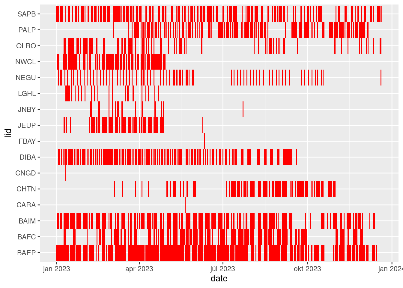
One way to think about this is if your boss was interested in the statistics of the sampling site visited by date over a year. The way to achieve this given the current datatable structure is to first get the distinct records of date and landings site:

table1 <- 
  d |> 
  # there is still some error in the date entry
  filter(year(date) == 2023) |> 
  select(date, lid) |>
  distinct() 
table1 |> 
  ggplot(aes(date, lid)) +
  geom_tile(fill = "red")