Catch Per Unit Effort (CPUE)
Definition
CPUE as an index of abundance
The use of CPUE as an index of abundance is based on a fundamental relationship widely used in quantitative fisheries analysis. The relationship relates catch to abundance and effort:
\[ C_t =qE_tN_t \]
Where \(C_t\) is catch at time \(t\); \(E_t\) is the effort expended at time \(t\); \(N_t\) is abundance at time \(t\); and \(q\) is the portion of the stock captured by one unit of effort (often called the catchability coefficient).
The equation can be rearranged to form the relationship between CPUE and abundance
\[ C_t/E_t = qN_t \]
making CPUE proportional to abundance, provided \(q\) is constant over time
\[ CPUE_t ∝ N_t \]
Is CPUE proportional to abundance
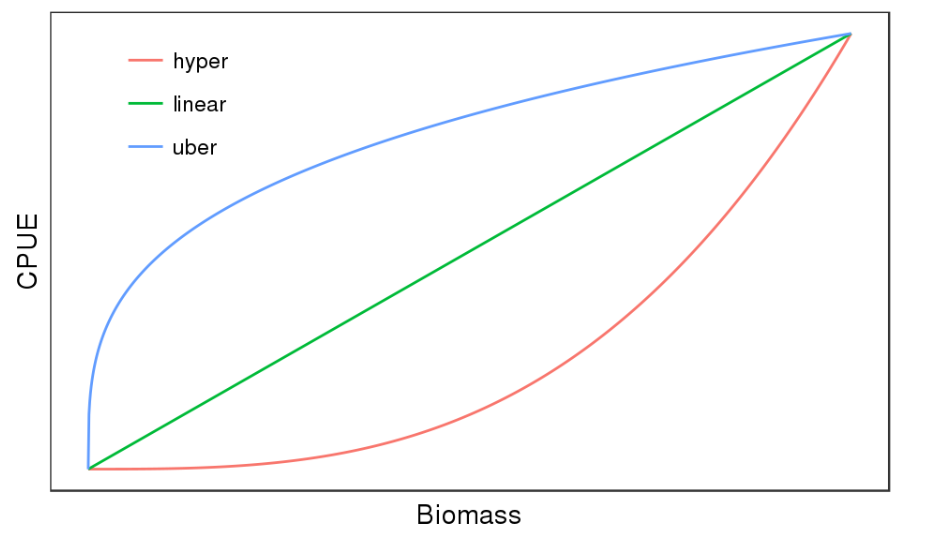
CPUE may not be directly related to biomass. Fishery dependent data can exhibit characteristics of preferential sampling.
The most common non-proportionality involves CPUE remaining high while abundance declines. This is known as “hyperstability” and can lead to overestimation of biomass and underestimation of fishing mortality or the opposite “hyperdepletion”.
Is q constant in time?
The fundamental assumption that \(q\) is constant in time needs to be met if \(CPUE\) is to tell us anything about stock dynamics.
Unfortunately \(q\) is seldom constant over the entire exploitation history; it can vary for many reasons. Some of the factors that commonly cause \(q\) to change over time are:
the change in the efficiency of the fleet
species targeting
the environment
dynamics of the population or fishing fleet
Efficiency of a fleet
Catchability often increases over time as the efficiency of the fleet increases.
The efficiency of a fleet can increase through:
fishers learning more about the location and behaviour of fish
how to operate gear more efficiently
Efficiency also increases when new technologies are obtained:
Fish finding devices
Navigation devices (GPS)
Fish aggregating devices (FAD)
Targeting by a fleet
The catchability of a species can be greatly affected when a fleet changes its targeting practice from one species to another.
In general, catchability increases for the new target species, and decreases for the previous target species.
Example from Japan:
- The increase in depth of longline gear to target bigeye tuna increased the catchability for that species, but decreased the catchability of longfin tuna.
Environmental factors
The environment can have a large influence on catchability.
For example, the 1981-1983 El Nino reduced catchability of yellowfin tuna to the purse seine fisheries of the eastern Pacific Ocean to such an extent that many vessels transferred their operations to the western Pacific.
Sometime migratory species can change behaviour or experience spatial range shifts that are climate driven and may not be found in their usual places.
Dynamics of a population or fleet
Catchabiltiy is often related to abundance, and abundance changes over time, so will catchability.
The definition of effort also matters.
For example, each set of a purse seine in the tuna fishery catches a school, and if the school size does not change with abundance, catch per set will remain the same. However, the time needed to find a school might change, so the measure of effort should be searching time, rather than the number of sets.
Many other factors that may influence the assumption of catchability being proportional to abundance: stock structure (harvesting multiple species together); age/size selectivity; gear saturation and interference; individual variability in natural mortality.
What portion of the stock does CPUE relate to?
CPUE measures only the component of the population that is vulnerable to the gear ; it may be proportional to this component of the population, but not to the total population
The proportion of the population that is vulnerable to the fishery depends on:
gear selectivity
size and age of fish
horizontal and vertical distribution of fish
fishing practice of the fleet
For example, a fishery may only catch adult fish if fishing operations are restricted to deep waters.
What portion of the stock does the CPUE relate to?
The amount of overlap of spatial distribution of the fish population and the fishing fleet can have a considerable influence on how cpue relates to abundance
If the fishery operates on only a fraction of the population and the mixing rates of fish among areas is low, there will be little relationship between cpue and total population abundance.
Despite tuna being regarded as highly migratory, movement of most fish is limited for species like yellowfin, skipjack, and bigeye tuna, and there is a distinct possibility of local depletion and different cpue trends in different parts of a very large ocean.
CPUE Standardization
What is it and why do we need it?
Rarely have independent population estimates of fish abundance
Rely on catch data for population trends to make management decisions
Multiple factors can contribute to variation:
Changes in effort (e.g. gear type)
Spatial effects (e.g. habitat quality)
Temporal effects (e.g. seasonal patterns or cycles)
Environmental effects (temperature/rainfall/upwelling, etc.)
Goal of standardization is to remove variation not due to changes in abundance to make CPUE proportional to abundance
Methods for CPUE Standardization
Many fishery systems are inherently nonlinear, and methods that can handle nonlinear relationships between catch rate and potential variables that capture changes over time and space in catchability may be more appropriate
Linear Mixed Models
Generalized Linear Models / Generalized Linear Mixed Models
Generalized Additive Models / Generalized Additive Mixed Models
Zero-inflated models
Spatial-temporal generalized linear mixed model (VAST R package) has great potential
Bayesian inference
And many other statistical tools …
Approach
Formulate the question
E.g. What variables contribute to variance in tuna catch?
Explore the data
Outliers, collinearity, Zeros, type of relationships
Do not ignore zeros! Often replaced with a small number or use an appropriate distribution to accommodate zeros
Model the data
- Model fitting, selection, validation, interpretation
Discuss findings
What does it mean?
Can the model be used for predicting an index of abundance?
Data exploration is a critical step
Before calculating any CPUE it is prudent to explore the catch/ logbook data and try to get an idea about the fishery . We need to look at:
Have there been changes in gear over year?
Has the spatial distribution changed?
Has the temporal seasonal pattern changed?
Has targetting changed?
Have there been changes in legistlation or market that may have affected the fishery?
Does our data have the statistical properties that are assumed in the standardising procedure?
Choice of explanatory variables
The standardization attempts should ensure that the \(q\) can be assumed to be constant ….
Varibles could be:
Type of trawl gear, Time of day
Vessel id, Vessel size (length, breadth)
Environmental factors (Sea surface Temperature SST)
YEAR , Area, month, catch or catch rates of other species….
The choice of a statistical distribution
The choice of a statistical distribution should take into account the nature of the data.
For example, a discrete distribution, such as the Poisson or the negative binomial, may be the most appropriate distribution if the catch is recorded in individuals. In this case, the catch, rather than the catch rate, should be the response variable, and the fishing effort should be included as an offset or perhaps as an explanatory variable
\[ log(Catch) = log(Effort) + Year + Area + ... \]
However, a continuous distribution can be used if the catch is in weight, catch rate is modeled, or a large number of individuals are usually caught by each unit of effort
\[ log(CPUE) = Year + Area + ... \]
It is however recommended to use the raw data (catch and effort).
Conclusion
CPUE is a very tricky data set to use in stock assessment:
Hard to standardize
Can give misleading information
Sometimes the only data we have
Therefore model formulation and interpretation needs to be followed cautiously!
Note
CPUE is not used on its own to draw inferences about population status, it gives you a standardized index of abundance that can then be used in a stock assessment model (such as Surplus production models e.g. CMSY (catch maximum sustainable yield) or SPiCT (surplus production models in continuous time which requires a larger data set than CSMY) to get your biological reference points \(B_{MSY}\) and \(F_{MSY}\).